1 Algorithm Analysis

[Definition] An algorithm is a finite set of instructions that, if followed, accomplishes a particular task. In addition, all algorithms must satisfy the following criteria.

Input : There are zero or more quantities that are externally supplied.
Output : At least one quantity is produced.
Definiteness : Each instruction is clear and unambiguous.
Finiteness : the algorithm terminates after finite number of steps
Effectiveness : basic enough to be carried out ; feasible

A program does not have to be finite. (eg. an operation system)
An algorithm can be described by human languages, flow charts, some programming languages, or pseudocode.

[Example] Selection Sort : Sort a set of $n\geq1$ integers in increasing order

for (i = 0; i < n; i++){
    Examine list[i] to list[n-1] and suppose that the smallest integer is at list[min];
    Interchange list[i] and list[min];
}

1.1 What to Analyze

Machine and compiler-dependent run times.
Time and space complexities : machine and compiler independent.
Assumptions:
1. instructions are executed sequentially 顺序执行
2. each instruction is simple, and takes exactly one time unit
3. integer size is fixed and we have infinite memory

$T_{avg}(N)\, and\, T_{worst}(N)$ : the average and worst case time complexities as functions of input size $N$

[Example] Matrix addition

void add(int a[][MAX_SIZE],
         int b[][MAX_SIZE],
         int c[][MAX_SIZE],
         int rows, int cols) 
{
    int i, j;
    for (i=0; i<rows; i++)/*rows+1*/
        for (j=0;j<cols;j++)/*rows(cols+1)*/
            c[i][j] = a[i][j]+b[i][j];/*rows*cols*/
}

$T(rows, cols) = 2rows\times cols + 2rows+1$

非对称

[Example] Iterative function for summing a list of numbers

float sum (float list[], int n)
{  /*add a list of numbers*/
    float tempsum = 0; /*count = 1*/
    int i;
    for (i=0; i<n; i++)
        /*count++*/
        tempsum  += list[i]; /*count++*/
    /*count++ for last excutaion of for*/
   return tempsum; /*count++*/
}

$T_{sum}(n)=2n+3$

[Example] Recursive function for summing a list of numbers

float rsum (float list[], int n)
{/*add a list of numbers*/
    if (n) /*count++*/
        return rsum(list, n-1) + list[n-1];
        /*count++*/
    return 0; /*count++*/
}

$T_{rsum}(n)=2n+2$

But it takes more time to compute each step.

1.2 Asymptotic Notation( $O,\Omega,\Theta,o$ )

predict the growth ; compare the time complexities of two programs ; asymptotic(渐进的) behavior

[Definition] $T(N)=O(f(N))$ if there are positive constants $c$ and $n_0$ such that $T(N)\leq c\cdot f(N)$ for all $N\geq n_0$ .(upper bound)

[Definition] $T(N)=\Omega(g(N))$ if there are positive constants $c$ and $n_0$ such that $T(N)\geq c\cdot f(N)$ for all $N\geq n_0$ .(lower bound)

[Definition] $T(N)=\Theta(h(N))$ if and only if $T(N)=O(h(N))$ and $T(N)=\Omega(h(N))$

[Definition] $T(N)=o(p(N))$ if $T(n)=O(p(N))$ and $T(N)\neq\Theta(p(N))$

$2N+3=O(N)=O(N^{k\geq1})=O(2^N)=\ldots$ take the smallest $f(N)$
$2^N+N^2=\Omega(2^N)=\Omega(N^2)=\Omega(N)=\Omega(1)=\ldots$ take the largest $g(N)$
Rules of Asymptotic Notation
1. If $T_1(N)=O(f(N))$ and $T_2=O(g(N))$ , then
  
  (1) $T_1(N)+T_2(N)=max(O(f(N)),O(g(N)))$
  
  (2) $T_1(N)*T_2(N)=O(f(N)*g(N))$
2. 若 $T(N)$ 是一个 $k$ 次多项式，则 $T(N)=\Theta(N^k)$
3. $log_kN=O(N^m)$ for any constant $k$ (logarithms grow very slowly)，无论k多小（当然要大于1），m多小（当然要大于等于0），这个式子都成立。

[Example] Matrix addition

void add(int a[][MAX_SIZE],
         int b[][MAX_SIZE],
         int c[][MAX_SIZE],
         int rows, int cols) 
{
    int i, j;
    for (i=0; i<rows; i++)
        for (j=0;j<cols;j++)
            c[i][j] = a[i][j]+b[i][j];
}

$T(rows,cols)=\Theta(rows\cdot cols)$

General Rules

For loops : The running time of a for loop is at most the running time of the statements inside the for loop (including tests) times the number of iterations.

Nested for loops : The total running time of a statement inside a group of nested loops is the running time of the statements multiplied by the product of the sizes of all the for loops.

Consecutive statements : These just add (which means that the maximum is the one that counts).

If/else : For the fragment
if ( Condition ) S1;
else S2;

The running time is never more than the running time of the test plus the larger of the running time of S1 and S2.
Recursions :

[Example] Fibonacci number

$Fib(0)=Fib(1)=1, Fib(n)=Fib(n-1)+Fib(n-2)$
1
2
3
4
5
6
7
long int Fib (int N) /*T(N)*/
{
    if (N<=1) /*O(1)*/
        return 1; /*O(1)*/
    else
        return Fib(N-1)+Fib(N-2);
}      /*O(1)*//*T(N-1)*//*T(N-2)*/
$T(N)=T(N-1)+T(N-2)+2\geq Fib(N)\\ \left(\frac{3}{2} \right)^n\leq Fib(N)\leq\left(\frac{5}{3}\right)^n$

时间复杂度： $O(2^N)$ $T(N)$ grows exponentially

空间复杂度： $O(N)$ 递归深度是最大深度，不是所有深度之和，因为上一次用的栈已经倍释放

如果是迭代的话时间为 $O(n)$ 空间为 $O(1)$

1.3 Compare the Algorithms

[Example] 最大子序列和

Algorithm 1

int  MaxSubsequenceSum ( const int A[ ],  int  N ) 
{ 
    int ThisSum, MaxSum, i, j, k; 
     MaxSum = 0;   /* initialize the maximum sum */
     for( i = 0; i < N; i++ )  /* start from A[ i ] */
         for( j = i; j < N; j++ ) {   /* end at A[ j ] */
             ThisSum = 0; 
             for( k = i; k <= j; k++ ) 
                 ThisSum += A[ k ];  /* sum from A[ i ] to A[ j ] */
             if ( ThisSum > MaxSum ) 
                   MaxSum = ThisSum;  /* update max sum */
        }  /* end for-j and for-i */
     return MaxSum; 
}

$T(N)=O(N^3)$

Algotithm 2

int  MaxSubsequenceSum ( const int A[ ],  int  N ) 
{ 
    int ThisSum, MaxSum, i, j; 
     MaxSum = 0;   /* initialize the maximum sum */
     for( i = 0; i < N; i++ ) {   /* start from A[ i ] */
         ThisSum = 0; 
         for( j = i; j < N; j++ ) {   /* end at A[ j ] */
             ThisSum += A[ j ];  /* sum from A[ i ] to A[ j ] */
             if ( ThisSum > MaxSum ) 
                   MaxSum = ThisSum;  /* update max sum */
        }  /* end for-j */
    }  /* end for-i */
     return MaxSum; 
}

$T(N)=O(N^2)$

Algorithm 3 Divide and Conquer 分治法

static int MaxSubSum(const int A[ ], int Left, int Right)
{
    int MaxLeftSum, MaxRightSum;
    int MaxLeftBorderSum, MaxRightBorderSum;
    int LeftBorderSum, RightBorderSum;
    int Center, i;
    
    if (Left == Right)
        if (A[Left] > 0)
            return A[Left];
        else
            return 0;
    
    Center = (Left + Right) / 2;
    MaxLeftSum = MaxSubSum(A, Left, Center);
    MaxRightSum = MaxSubSum(A, Center + 1, Right);
    
    MaxLeftBorderSum = 0;
    LeftBorderSum = 0;
    for (i = Center; i >= Left; i--)
    {
        LeftBorderSum += A[i];
        if (LeftBorderSum > MaxLeftBorderSum)
            MaxLeftBorderSum = LeftBorderSum;
    }
    
    MaxRightBorderSum = 0;
    RightBorderSum = 0;
    for (i = Center+1; i <= Right; i++)
    {
        RightBorderSum += A[i];
        if (RightBorderSum > MaxRightBorderSum)
            MaxRightBorderSum = RightBorderSum;
    }
    
    return Max3(MaxLeftSum, MaxRightSum, MaxLeftBorderSum + MaxRightBorderSum);
}

int MaxSubsequenceSum(const int A[ ], int N)
{
    return MaxSubSum(A, 0, N - 1);
}

$\because T(N)=2T(\frac N2)+cN\quad T(1)=O(1)\\ T(\frac N2)=2T(\frac N {2^2})+c\frac N2\\ \cdots \\ T(1)=2T(\frac N{2^k})+c\frac N{2^{k-1}} \\ \therefore T(N)=2^kT(\frac N{2^k})+kcN=N\cdot O(1)+cN\log N$

Algorithm 4 On-line Algorithm 在线算法

int MaxSubsequenceSum( const int  A[ ],  int  N ) 
{ 
    int ThisSum, MaxSum, j; 
     ThisSum = MaxSum = 0; 
     for ( j = 0; j < N; j++ ) { 
         ThisSum += A[ j ]; 
         if ( ThisSum > MaxSum ) 
             MaxSum = ThisSum; 
         else if ( ThisSum < 0 ) 
             ThisSum = 0;
    }  /* end for-j */
     return MaxSum; 
}

$T(N)=O(N)$

A[ ] is scanned once only. 扫描一次，无需存储（处理streaming data）
在任意时刻，算法都能对它已经读入的数据给出子序列问题的正确答案(其他算法不具有这个特性)

1.4 Logrithms in the Running Time

如果一个算法用常数时间将问题的大小削减为其一部分(通常是1/2)，那么该算法就是 $O(logN)$ 的

[Example] Binary Search

int BinarySearch ( const ElementType A[ ], ElementType X, int N ) 
{ 
    int  Low, Mid, High; 
     Low = 0;  High = N - 1; 
     while ( Low <= High ) { 
         Mid = ( Low + High ) / 2; 
         if ( A[ Mid ] < X ) 
             Low = Mid + 1; 
        else 
             if ( A[ Mid ] > X ) 
                 High = Mid - 1; 
            else 
                 return  Mid; /* Found */ 
    }  /* end while */
     return  NotFound; /* NotFound is defined as -1 */ 
}

$T_{worst}(N)=O(\log N)$

[Example] Euclid’s Algorithm

int Gcd(int M, int N)
{
    int Rem;
    
    while (N > 0)
    {
        Rem = M % N;
        M = N;
        N = Rem;
    }
    return M;
}

[Example] Efficient exponentiation

long int Pow(long int X, int N)
{
    if (N == 0) return 1;
    if (N == 1) return X;
    if (IsEven(N)) return Pow(X*X, N/2);/*return Pow(X, N/2)*Pow(X, N/2) affects the efficiency*/
    else return Pow(X*X, N/2)*X; /*return Pow(X, N-1)*X is the same*/
}

1.5 Checking Your Analysis

Method 1

When $T(N)=O(N)$ , check if $T(2N)/T(N)\approx2$

When $T(N)=O(N^2)$ , check if $T(2N)/T(N)\approx4$

When $T(N)=O(N^3)$ , check if $T(2N)/T(N)\approx8$

Method 2

When $T(N)=O(f(N))$ , check if $\lim\limits_{N\rightarrow\infty}\frac{T(N)}{f(N)}\approx C $

2 LIst, Stacks and Queues

2.1 Abstract Data Type(ADT) 抽象数据类型

[Definition] Data Type = {Objects} and {Operations}

[Definition] An Abstract Data Type(ADT) is a data type that is organized in such a way that the specification on the objects and specification of the operations on the objects are separated from the representation of the objects and the implementation on the operations.

2.2 The List ADT

Objects : N items
Operations
- Finding the length
- Printing
- Making an empty
- Finding
- Inserting
- Deleting
- Finding next
- Finding previous

Simple Array implementation of Lists

Sequential mapping 连续存储，访问快
Find_Kth take $O(1)$ time.
MaxSize has to be estimated.
Insertion and Deletion not only take $O(N)$ times, but also involve a lot of data movements which takes time. 访问要 $O(1)$ ，插入要 $O(N)$ 。如果要随机访问的话，肯定是线性表最快。

Query 查询

Linked Lists

Location of nodes may change on differrent runs.
Insertion 先连后断
Deletion 先连后释放
频繁malloc和free系统开销较大

Finding take $O(N)$ times.

/*Return true if L is empty*/
int IsEmpty(List L)
{
    return L->Next == NULL;
}

/*Return true if P is the last position in list L*/
/*Parameter L is unused in this implementation*/
int IsLast(Position P, List L)
{
    return P->Next == NULL;
}

/*Return Position of X in L; NULL if not found*/
Position Find(Element X, List L)
{
    Position P;
    
    P = L->Next;
    while (P != NULL && P->Element != X) P = P->Next;
    
    return P;
}

/*Delete first occurence of X from a list*/
/*Assume use of a header node*/
void Delete(ElementType X, List L)
{
    Position P, TmpCell;
    
    P = FindPrevious(X, L);
    
    if (!IsLast(P, L))
    {
        TmpCell = P->Next;
        P->Next = TmpCell->Next;
        free(TmpCell);
    }
}

/*If X is not found, then Next field of returned*/
/*Assumes a header*/
Position FindPrevious(ElementType X, List L)
{
    Position P;
    
    P = L;
    while (P->Next != NULL && P->Next->Element != X) P = P->Next;
    
    return P;
}

/*Insert (after legal position P)*/
/*Header implementation assumed*/
/*Parameter L is unused in this implementation*/
void Insert(ElementType X, List L, Position P)
{
    Position TmpCell;
    
    TmpCell = malloc(sizeof(struct Node));
    if (TmpCell == NULL) FatalError("Out of space!")
    
    TmpCell->Element = X;
    TmpeCell->Next = P->Next;
    P->Next = TmpCell;
}

void DeleteList(List L)
{
    Position P, Tmp;
    
    P = L->Next;
    L->Next = NULL;
    while (P != NULL)
    {
        Tmp = P->Next;
        free(P);
        P = Tmp;
    }
}

Doubly Linked Circular Lists

Finding take $O(\frac N 2)$ times.

The correct answer is D.

Two Applications

The Polynomial ADT

Objects :
Operations :
- Finding degree
- Addition
- Subtraction
- Multiplication
- Differentiation

[Representation 1]

typedef struct {
    int CoeffArray [ MaxDegree + 1 ] ;
    int HighPower;
}  *Polynomial ;

/*将多项式初始化为零*/
void ZeroPolynomial(Polynomial Poly)
{
    int i;
    for(i = O; i <= MaxDegree; i++)
        Poly->CoeffArray[ i ] = O;
    Poly->HighPower = O;
}

/*两个多项式相加*/
void AddPolynomial(const Polynomial Poly1, const Polynomial Poly2, Polynomial PolySum)
{
    int i;
    
    ZeroPolynomial(PolySum);
    PolySum->HighPower = Max(Poly1->HighPower, Poly2->HighPower);
    
    for (i = PolySum->HighPower; i >= O; i--)
        PolySum->CoeffArray[ i ] = Poly1->CoeffArray[ i ] + Poly2->CoeffArray[ i ];
}

void MultPolynomial(const Polynomial Poly1, const Polynomial Poly2, Polynomial PolyProd)
{
    int i, j;
    
    ZeroPolynomial (PolyProd);
    PolyProd->HighPower = Poly1->HighPower + Poly2->HighPower;
    
    if(PolyProd->HighPower > MaxDegree)
        Error("Exceeded array size");
    else
        for(i = O; i <= Poly1->HighPower; i++)
            for(j = O; j <= Poly2->HighPower; j++)
                PolyProd->CoeffArray[ i + j ] += Poly1->CoeffArray[ i ] * Poly2->CoeffArray[ j ];
}

[Representation 2]

typedef struct poly_node *poly_ptr;
struct poly_node{
    int Coefficient;  /* assume coefficients are integers */
    int Exponent;
    poly_ptr Next;
};
typedef poly_ptr a;    /* nodes sorted by exponent */

只存储非零项

Multilists

Cursor Implementation of Linked Lists(no pointer)

2.3 The Stack ADT

Last-In-First-Out (LIFO)
Objects : A finite ordered list with zero or more elements.
Operations :
- IsEmpty
- CreatStack
- DisposeStack
- MakeEmpty
- Push
- Top
- Pop
A Pop(or Top) on an empty stack in an error in the stack ADT.
Push on a full stack is an implementation error but not an ADT error.
如果考那种算数式子的入栈出栈的话，符号是不用入栈的；但是如果题目要求用栈实现算式从中序变成post就是需要的，而且左右括号也是算进栈的空间的！

Linked List Implementation (with a header node)

3-1

The calls to malloc and free are expensive. Simply keep another stack as a recycle bin.

int IsEmpty(Stack S)
{
    return S->Next == NULL;
}

Stack CreateStack(void)
{
    Stack S;
    S = malloc(sizeof(struct Node));
    if (S == NULL)
        Fatal Error("Out of space!");
    S->Next == NULL;
    MakeEmpty(S);
    return S;
}

void MakeEmpty(Stack S)
{
    if (S == NULL)
        Error("Must use CreateStack first");
    else
        while(!IsEmpty(S)) Pop(S);
}

void Push(ElementType X, Stack S)
{
    PtrToNode TmpCell;
    TmpCell = malloc(sizeof(struct Node));
    if (TmpCell == NULL)
        Fatal Error("Out of space!") ;
    else
    {
        TmpCell->Element = X;
        TmpCe11->Next = S->Next;
        S->Next = TmpCell;
    }
}

ElementType Top(Stack S)
{
    if(!IsEmpty(S))
        return S->Next->Element;
    Error("Empty stack") ;
    return O; /* Return value used to avoid warning*/
}

void Pop(Stack s)
{
    PtrToNode FirstCell;
    if(IsEmpty(S))
        Error("Empty stack") ;
    else
    {
        FirstCe11 = S->Next;
        S->Next = S->Next->Next;
        free(FirstCe11);
    }
}

Array Implementation of Stacks

struct StackRecord {
    int Capacity;          /* size of stack */
    int TopOfStack;        /* the top pointer */
    /* ++ for push, -- for pop, -1 for empty stack */
    ElementType *Array;    /* array for stack elements */
};

The stack model must be well encapsulated(封装). That is, no part of your code, except for the stack routines, can attempt to access the Array or TopOfStack variable.

Error check must be done before Push or Pop (Top).

Stack CreateStack(int MaxElements)
{
    Stack S;
    if(MaxElements < MinStackSize)
    Error("Stack size is too small") ;
    S = malloc(sizeof(struct StackRecord));
    if (S == NULL)
        Fatal Error("Out of space!!!") ;

    S->Array = malloc(sizeof(ElementType) * MaxElements) ;
    if(S->Array = NULL)
        Fatal Error("Out of space!!!");
    S->Capacity = MaxElements;
    MakeEmpty(S) ;
    return S;
}

void DisposeStack(Stack S)
{
    if(S != NULL)
    {
        free(S->Array);
        free(S);
    }
}

int IsEmpty(Stack S)
{
    return S->TopOfStack == EmptyTOS;
}

void MakeEmpty(Stack S)
{
    S->TopOfStack = EmptyTOS;
}

void Push(ElementType X, Stack S)
{
    if (IsFull(S))
        Error("Full stack");
    else
        S->Array[ ++S->TopOfStack ] = X;
}

ElementType Top(Stack S)
{
    if(! IsEmpty(S))
        return S->Array[ S->TopOfStack ];
    Error("Empty stack") ;
    return O; /* Return value used to avoid warning*/
}

void Pop(Stack S)
{
    if(IsEmpty(S))
        Error("Empty stack") ;
    else
        S->TopOfStack--;
}

ElementType TopAndPop(Stack S)
{
    if(!Is Empty(S))
        return S->Array[ S->TopOfStack-- ];
    Error("Empty stack");
    return O; /* Return value used to avoid warnin */
}

Application

Balancing Symbols

检查括号是否平衡

Algorithm  {
    Make an empty stack S;
    while (read in a character c) {
        if (c is an opening symbol)
            Push(c, S);
        else if (c is a closing symbol) {
            if (S is empty)  { ERROR; exit; }
            else  {  /* stack is okay */
                if  (Top(S) doesn’t match c)  { ERROR, exit; }
                else  Pop(S);
            }  /* end else-stack is okay */
        }  /* end else-if-closing symbol */
    } /* end while-loop */ 
    if (S is not empty)  ERROR;
}

Postfix Evaluation 后缀表达式
Infix to Postfix Conversion
- 读到一个操作数时立即把它放到输出中
- 读到一个操作符时从栈中弹出栈元素直到发现优先级更低的元素为止，再将操作符压入栈中，注意最后一次右括号是不用入栈的，把两括号里面的通通弹出去就行了，括号是不用显示在输出中的，但是也占据栈的空间。
- The order of operands is the same in infix and postfix.
- Operators with higher precedence appear before those with lower precedence.
- Never pop a ’(‘ from the stack except when processing a ‘)’.
- When ‘(’ is not in the stack, its precedence is the highest; but when it is in the stack, its precedence is the lowest.
- Exponentiation associates right to left.
Function Calls (System Stack)

Note : Recursion can always be completely removed. Non recursive programs are generally faster than equivalent recursive programs. However, recursive programs are in general much simpler and easier to understand.

2.4 The Queue ADT

First-In-First-Out (FIFO)
Objects : A finite ordered list with zero or more elements.
Operations :
- IsEmpty
- CreatQueue
- DisposeQueue
- MakeEmpty
- Enqueue
- Front
- Dequeue

Array Implementation of Queues

struct QueueRecord {
    int Capacity ;       /* max size of queue */
    int Front;           /* the front pointer */
    int Rear;            /* the rear pointer */
    int Size;            /* Optional - the current size of queue */
    ElementType *Array;  /* array for queue elements */
 };

Circular Queue :

3-3 3-4

The maximum capacity of this queue is 5.
PPT中队列的初始化front = -1, rear = 0代表队列为空；在循环队列中如果不做处理，front = rear的时候就不知道是已经满了还是只有一个元素，一般的操作是在front前空一格元素，在初始化的时候把front弄成n - 1。
当然传统方法是把rear弄成队列末元素的下一个空格的下标的，这样初始化就变成了front = rear = 0. 判断是否满队可以用(front + 1) % maxSize == rear来判断；队列的长度可以用(rear - front + maxSize) % maxSize来计算。

Note : Adding a Size field can avoid wasting one empty space to distinguish “full” from “empty”.

3 Trees

3.1 Preliminaries

[Definition] A tree is a collection of nodes. The collection can be empty; otherwise, a tree consists of (1) a distinguished node r, called the root; (2) and zero or more nonempty (sub)trees, each of whose roots are connected by a directed edge from r.

Subtrees must not connect together. Therefore every node in the tree is the root of some subtree.
There are N-1 edges in a tree with N nodes

Terminologies

degree of a node : 结点的子树个数

degree of a tree : 结点的度的最大值

parent : 有子树的结点

children : the roots of the subtrees of a parent

siblings : children of the same parent

leaf(terminal node) : a node with degree 0(no children)

path from $n_1$ to $n_k$ : a unique sequence of nodes $n_1,n_2,\cdots,n_k$ such that $n_i$ is the parent of $n_{i+1}$ for $1\leq i<k$

length of path : 路径上边的条数

depth of $n_i$ : 从根结点到 $n_i$ 结点的路径的长度( $Depth(root)=0$ )

height of $n_i$ : 从 $n_i$ 结点到叶结点的最长路径的长度( $Height(leaf)=0$ )

height/depth of a tree : 根结点的高度/最深的叶结点的深度

ancestors of a node : 从此结点到根结点的路径上的所有结点

descendants of a node : 此结点的子树中的所有结点

List Representation

The size of each node depends on the number of branches.

The correct answer is T.

FirstChild-NextSibling Representation

The representation is not unique since the children in a tree can be of any order.

他也没说左边那个一定是FirstChild，所以是完全可以不唯一的。
注意如果一棵普通的T通过这个变换变成了BT，那么两者的前序遍历不变，且BT的中序遍历和T的后序遍历一样。

3.2 Binary Trees

[Definition] A binary tree is a tree in which no node can have more than two children.

Tree Traversals (visit each node exactly once)

Preorder Traversal

void preorder( tree_ptr tree )
{ 
    if( tree )   
    {
        visit ( tree );
        for (each child C of tree )
            preorder ( C );
    }
}

Postorder Traversal

void postorder( tree_ptr tree )
{  
    if( tree )   
    {
        for (each child C of tree )
            postorder ( C );
        visit ( tree );
    }
}

Levelorder Traversal

void levelorder( tree_ptr tree )
{   
    enqueue ( tree );
    while (queue is not empty) 
    {
        visit ( T = dequeue ( ) );
        for (each child C of T )
            enqueue ( C );
    }
}

Inorder Traversal

void inorder( tree_ptr  tree )
{  
     if( tree )   
    {
        inorder ( tree->Left );
         visit ( tree->Element );
         inorder ( tree->Right );
   }
}

Iterative Program :

void iter_inorder( tree_ptr tree )
{ 
    Stack  S = CreateStack( MAX_SIZE );
    for ( ; ; )  
    {
        for ( ; tree; tree = tree->Left )
            Push ( tree, S );
         tree = Top ( S );  
         Pop( S );
         if ( !tree ) break;
         visit ( tree->Element );
         tree = tree->Right; 
    }
}

4-3

注意：通过前序遍历和后序遍历在一定情况下是可以建树的！！别想当然以为给出的树会是三角形的。。。很有可能推出来就是一条线。。。

Threaded Binary Trees

A full binary tree with $n$ nodes has $2n$ links, and $n+1$ of them are NULL.
注意满二叉树(Full Binary Tree)是完全满的树，完全二叉树(Complete Binary Tree)是先填上层再填下层，同一层内先填左边后填右边的二叉树，不要搞混了。
Replace the NULL links by “threads” which will make traversals easier.

注意，这里如果左边或者右边已经都有非空指针了就不需要线索了。线索二叉树只是利用原来为空的结点进行一番操作。而且如果没有前驱或后继，这根指向NULL的线索是不能省去的！！

3-5

Rules :

If Tree->Left is null, replace it with a pointer to the inorder predecessor(中序前驱) of Tree.

If Tree->Right is null, replace it with a pointer to the inorder successor(中序后继) of Tree.

There must not be any loose threads. Therefore a threaded binary tree must have a head node of which the left child points to the first node.

typedef struct ThreadedTreeNode *PtrToThreadedNode;
typedef struct PtrToThreadedNode ThreadedTree;
typedef struct ThreadedTreeNode 
{
    int LeftThread;        /* if it is TRUE, then Left */
    ThreadedTree Left;     /* is a thread, not a child ptr.*/
    ElementType	Element;
    int RightThread;       /* if it is TRUE, then Right */
    ThreadedTree Right;    /* is a thread, not a child ptr.*/
}

线索化的实质就是将二叉链表中的空指针改为指向前驱或后继的线索。由于前驱和后继信息只有在遍历该二叉树时才能得到，所以，线索化的过程就是在遍历的过程中修改空指针的过程。看清楚他要的是什么遍历的线索二叉树，一般没说的话默认中序的。
In a tree, the order of children does not matter. But in a binary tree, left child and right child are different.

Properties of Binary Trees

The maximum number of nodes on level $i$ is $2^{i-1},i\geq1$ .

The maximum number of nodes in a binary tree of depth $k$ is $2^k-1,k\geq1$ .

For any nonempty binary tree, $n_0 = n_2 + 1$ where $n_0$ is the number of leaf nodes and $n_2$ is the number of nodes of degree 2.

推导（degree更多的同理）：

树的总顶点数 $v = n_0 + n_1 + n_2$ ，其中 $n_i$ 代表有 $i$ 个degree的顶点数；

每个顶点上方下方都有degree条边，即边的数量 $e = n_1 + 2n_2$ ，又有树中恒存在 $v = e + 1$ ，两个式子等一下就行了。

感觉考试的时候必考一道判断或者选择。

3.3 Binary Search Trees

[Definition] A binary search tree is a binary tree. It may be empty. If it is not empty, it satisfies the following properties:

每个结点有一个互不不同的值
若左子树非空，则左子树上所有结点的值均小于根结点的值
若右子树非空，则右子树上所有结点的值均大于根结点的值
左、右子树也是是一棵二叉查找树
给出互不相同的元素个数 $n$ ，能得到的不同的BST个数符合卡特兰数，通项公式为 $c_{n+1} = \frac{2(2n+1)}{n+2}\cdot c_n$ ，其中 $c_1 = 1, c_2 = 2, c_3 = 5, c_4 = 14 \cdots$ 这样。
假设在BST中同时有5，6，7三个数，6并不一定会是5、7两个点的parent，有可能5、7两个点分属两个不同的子树，6只是它们的ancestor.

ADT

Objects : A finite ordered list with zero or more elements.
Operations :
- SearchTree MakeEmpty( SearchTree T )
- Position Find( ElementType X, SearchTree T )
- Position FindMin( SearchTree T )
- Position FindMax( SearchTree T )
- SearchTree Insert( ElementType X, SearchTree T )
- SearchTree Delete( ElementType X, SearchTree T )
- ElementType Retrieve( Position P )

Implementations

Find

Position Find( ElementType X, SearchTree T ) 
{ 
    if ( T == NULL ) 
        return NULL;  /* not found in an empty tree */
    if ( X < T->Element )  /* if smaller than root */
        return Find( X, T->Left );  /* search left subtree */
    else 
        if ( X > T->Element )  /* if larger than root */
              return  Find( X, T->Right );  /* search right subtree */
        else   /* if X == root */
              return  T;  /* found */
}

$T(N)=S(N)=O(d)$ where $d$ is the depth of X

Iterative program :

Position Iter_Find( ElementType X, SearchTree T ) 
{ 
    while ( T )
    {
        if ( X == T->Element )  
            return T;  /* found */
        if ( X < T->Element )
            T = T->Left; /*move down along left path */
        else
             T = T-> Right; /* move down along right path */
    }  /* end while-loop */
    return NULL;   /* not found */
}

FindMin

Position FindMin( SearchTree T ) 
{ 
    if ( T == NULL )   
        return NULL; /* not found in an empty tree */
    else 
        if ( T->Left == NULL ) return T;  /* found left most */
        else return FindMin( T->Left );   /* keep moving to left */
}

FindMax

Position FindMax( SearchTree T ) 
{ 
    if ( T != NULL ) 
        while ( T->Right != NULL )   
            T = T->Right;   /* keep moving to find right most */
    return T;  /* return NULL or the right most */
}

Insert

SearchTree Insert( ElementType X, SearchTree T ) 
{ 
    if ( T == NULL ) /* Create and return a one-node tree */ 
    { 
        T = malloc( sizeof( struct TreeNode ) ); 
        if ( T == NULL ) 
            FatalError( "Out of space!!!" ); 
        else 
        { 
            T->Element = X; 
            T->Left = T->Right = NULL; 
        } 
    }  /* End creating a one-node tree */
    else  /* If there is a tree */
         if ( X < T->Element ) 
               T->Left = Insert( X, T->Left ); 
        else 
               if ( X > T->Element ) 
                  T->Right = Insert( X, T->Right ); 
           /* Else X is in the tree already; we'll do nothing */ 
    return  T;   /* Do not forget this line!! */ 
}

内存越界后不会马上报错，在下一次free或malloc时会失败
Handle duplicated keys
$T(N)=O(d)$

Delete

Delete a leaf node : Reset its parent link to NULL
Delete a degree 1 node : Replace the node by its single child
Delete a degree 2 node : 用左子树最大值结点或右子树最小值结点替换

SearchTree Delete( ElementType X, SearchTree T ) 
{    
    Position TmpCell; 
    if ( T == NULL ) Error( "Element not found" ); 
    else if ( X < T->Element )  /* Go left */ 
        T->Left = Delete( X, T->Left ); 
    else if ( X > T->Element )  /* Go right */ 
        T->Right = Delete( X, T->Right ); 
    else  /* Found element to be deleted */ 
        if ( T->Left && T->Right ) {  /* Two children */ 
        /* Replace with smallest in right subtree */ 
            TmpCell = FindMin( T->Right ); 
            T->Element = TmpCell->Element; 
            T->Right = Delete( T->Element, T->Right );  } /* End if */
        else 
        {  /* One or zero child */ 
            TmpCell = T; 
            if ( T->Left == NULL ) /* Also handles 0 child */ 
                T = T->Right; 
            else if ( T->Right == NULL )  
                T = T->Left; 
            free( TmpCell );  
         }  /* End else 1 or 0 child */
      return  T; 
}

$T(N)=O(d)$

Note : If there are not many deletions, then lazy deletion may be employed: add a flag field to each node, to mark if a node is active or is deleted. Therefore we can delete a node without actually freeing the space of that node. If a deleted key is reinserted, we won’t have to call malloc again.

Average-Case Analysis
- The average depth over all nodes in a tree is $O(logN)$ on the assumption that all trees are equally likely.
- 将 $n$ 个元素存入二叉搜索树，树的高度将由插入序列决定

The correct answer is A.

4 Priority Queues (Heaps)

4.1 ADT Model

Objects :A finite ordered list with zero or more elements.
Operations :
- PriorityQueue Initialize( int MaxElements );
- void Insert( ElementType X, PriorityQueue H );
- ElementType DeleteMin( PriorityQueue H );
- ElementType FindMin( PriorityQueue H );

4.2 Implementations

Array

Insertion — add one item at the end ~ $\Theta(1)$
Deletion — find the largest / smallest key ~ $\Theta(n)$

remove the item and shift array ~ $O(n)$

Linked List

Insertion — add to the front of the chain ~ $\Theta(1)$
Deletion — find the largest / smallest key ~ $\Theta(n)$

remove the item ~ $\Theta(1)$

Never more deletions than insertions

Ordered Array

Insertion — find the proper position ~ $O(\log n)$

shift array and add the item ~ $O(n)$
Deletion — remove the first / last item ~ $\Theta(1)$

Ordered Linked List

Insertion — find the proper position ~ $O(n)$

add the item ~ $\Theta(1)$
Deletion — remove the first / last item ~ $\Theta(1)$

Binary Search Tree

Both insertion and deletion will take $O(\log N)$ only.
Only delete the the minimum element, always delete from the left subtrees.
Keep a balanced tree
But there are many operations related to AVL tree that we don’t really need for a priority queue.

4.3 Binary Heap

Structure Property

[Definition] A binary tree with $n$ nodes and height $h$ is complete if its nodes correspond to the nodes numbered from $1$ to $n$ in the perfect binary tree of height $h$ .

A complete binary tree of height $h$ has between $2^h$ and $2^{h+1}-1$ nodes.
$h=\lfloor\log N\rfloor$
Array Representation : BT[n + 1] ( BT[0] is not used)

[Lemma]

$index\,of\,parent(i)=\left\{ \begin{array}{rcl} \lfloor i/2\rfloor && {i\neq1}\\ None && {i=1}\\ \end{array} \right.$
$index\,of\,left\_child(i)=\left\{ \begin{array}{rcl} 2i && {2i\leq n}\\ None && {2i>n}\\ \end{array} \right.$
$index\,of\,right\_child(i)=\left\{ \begin{array}{rcl} 2i+1 && {2i+1\leq n}\\ None && {2i+1>n}\\ \end{array} \right.$

PriorityQueue Initialize( int MaxElements ) 
{ 
    PriorityQueue H; 
    if ( MaxElements < MinPQSize ) 
        return Error( "Priority queue size is too small" ); 
    H = malloc(sizeof( struct HeapStruct )); 
    if ( H == NULL ) 
        return FatalError( "Out of space!!!" ); 
    /* Allocate the array plus one extra for sentinel */ 
    H->Elements = malloc(( MaxElements + 1 ) * sizeof( ElementType )); 
    if ( H->Elements == NULL ) 
        return FatalError( "Out of space!!!" ); 
    H->Capacity = MaxElements; 
    H->Size = 0; 
    H->Elements[0] = MinData;  /* set the sentinel */
    return H; 
}

Heap Order Property

[Definition] A min tree is a tree in which the key value in each node is no larger than the key values in its children (if any). A min heap is a complete binary tree that is also a min tree.

We can declare a max heap by changing the heap order property.

Basic Heap Operations

Insertion

/*H->Element[ 0 ] is a sentinel that is no larger than the minimum element in the heap.*/ 
void Insert( ElementType X, PriorityQueue H ) 
{ 
    int i; 
    if ( IsFull( H )) 
    { 
        Error( "Priority queue is full" ); 
        return; 
    } 
    for ( i = ++H->Size; H->Elements[ i/2 ] > X; i /= 2 ) 
        H->Elements[ i ] = H->Elements[ i/2 ]; /*Percolate up, faster than swap*/
    H->Elements[ i ] = X; 
}

$T(N)=O(\log N)$

DeleteMin

ElementType DeleteMin( PriorityQueue H ) 
{ 
    int i, Child; 
    ElementType MinElement, LastElement; 
    if ( IsEmpty( H ) ) 
    { 
        Error( "Priority queue is empty" ); 
        return H->Elements[ 0 ];   
    } 
    MinElement = H->Elements[ 1 ];  /*Save the min element*/
    LastElement = H->Elements[ H->Size-- ];  /*Take last and reset size*/
    for ( i = 1; i * 2 <= H->Size; i = Child )  /*Find smaller child*/ 
    {
        Child = i * 2; 
        if (Child != H->Size && H->Elements[Child+1] < H->Elements[Child]) 
               Child++;     
        if ( LastElement > H->Elements[ Child ] )   /*Percolate one level*/ 
                H->Elements[ i ] = H->Elements[ Child ]; 
        else     
            break;   /*Find the proper position*/
    } 
    H->Elements[ i ] = LastElement; 
    return MinElement; 
}

$T(N)=O(\log N)$

Other Heap Operations

查找除最小值之外的值需要对整个堆进行线性扫描

DecreaseKey — Percolate up
IncreaseKey — Percolate down
Delete
BuildHeap

将N 个关键字以任意顺序放入树中，保持结构特性，再执行下滤
1
2
for (i = N/2; i > 0; i--)
PercolateDown(i);
$T(N)=O(N)$

[Theorem] For the perfect binary tree of height $h$ containing $2^{h+1}-1$ nodes, the sum of the heights of the nodes is $2^{h+1}-1-(h+1)$ .

感觉这道题错了好几次了，如果每两层之间应该是需要两次，因为子节点之间需要比一次，当前结点与子节点的小的那个又要比一次，就要 $2\cdot (2^{h+1}-1-(h+1))$ 次比较了，把 $N \approx 2^{h + 1} - 1$ 代进去，得到的结果是 $2\cdot (N - \log(N + 1))$ 次比较。

4.4 Applications of Priority Queues

Heap Sort

查找一个序列中第k小的元素

The function is to find the K-th smallest element in a list A of N elements. The function BuildMaxHeap(H, K) is to arrange elements H[1] … H[K] into a max-heap.

ElementType FindKthSmallest ( int A[], int N, int K )
{   /* it is assumed that K<=N */
    ElementType *H;
    int i, next, child;

    H = (ElementType*)malloc((K+1)*sizeof(ElementType));
    for ( i = 1; i <= K; i++ ) H[i] = A[i-1];
    BuildMaxHeap(H, K);

    for ( next = K; next < N; next++ ) {
        H[0] = A[next];
        if ( H[0] < H[1] ) {
            for ( i = 1; i*2 <= K; i = child ) {
                child = i*2;
                if ( child != K && H[child+1] > H[child] ) child++;
                if ( H[0] < H[child] )
                    H[i] = H[child];
                else break;
            }
            H[i] = H[0];
        }
    }
    return H[1];
}

4.5 $d$ -Heaps — All nodes have $d$ children

Note :

DeleteMin will take $d-1$ comparisons to find the smallest child. Hence the total time complexity would be $O(d \log_d N)$ .

*2 or /2 is merely a bit shift, but *d or /d is not.

When the priority queue is too large to fit entirely in main memory, a d-heap will become interesting.

正确答案是4，注意“in the process”

5 The Disjoint Set

5.1 Equivalence Relations

[Definition] A relation, ~, over a set, S, is said to be an equivalence relation over S if it is symmetric, reflexive, and transitive over S.

[Definition] Two members x and y of a set S are said to be in the same equivalence class if x ~ y.

5.2 The Dynamic Equivalence Problem

Given an equivalence relation ~, decide for any a and b if a ~ b

Algorithm: (Union/Find)
{
    /* step 1: read the relations in */
    Initialize N disjoint sets;
    while ( read in a ~ b )
    {
        if ( !(Find(a) == Find(b)) )  /*Dynamic(on-line)*/
            Union the two sets;
    } /* end-while */
    /* step 2: decide if a ~ b */
    while ( read in a and b )
        if ( Find(a) == Find(b) )
            output( true );
        else   
            output( false );
}

Elements of the sets : $1,2,3,\cdots,N$
Sets : $S_1,S_2,\cdots\,and\,S_i\bigcap S_j=\emptyset\,(if\quad i\neq j)$
Operations :
- Union( $i, j$ ) = Replace $S_i$ and $S_j$ by $S=S_i\bigcup S_j$
- Find( $i$ ) = Find the set $S_k$ which contains the element $i$

5.3 Basic Data Structure

Union( $i, j$ )

Make $S_i$ a subtree of $S_j$ , or vice versa, that is to set the parent pointer of one of the roots to the other root.
Implementation 1 :
Implementation 2 :
- The elements are numbered from 1 to N, hence they can be used as indices of an array.
- S[ element ] = the element’s parent
- Note : S[ root ] = 0 and set name = root index
- 数组初始化全部为0
1
2
3
4
void SetUnion(DisjSet S, SetType Rt1, SetType Rt2)
{
S[Rt2] = Rt1;
}

Find( $i$ )

Implementation 1 :

Implementation 2 :

SetType Find(ElementType X, DisjSet S)
{
    for ( ; S[X]>0; X=S[X]);
    return X;
}

Analysis

Union and find are always paired. Thus we consider the performance of a sequence of union-find operations.

Algorithm using union-find operations:
{  
    Initialize Si = { i }  for  i = 1, ..., 12 ;
    for ( k = 1; k <= 9; k++ )  /* for each pair i R j */
    {
        if ( Find( i ) != Find( j ) )
            SetUnion( Find( i ), Find( j ) );
    }
}

Worst case : $T(N)=\Theta(N^2)$

5.4 Smart Union Algorithms

Union-by-Size

Always change the smaller tree
S[Root] = -size, initialized to be -1
[Lemma] Let T be a tree created by union-by-size with N nodes, then $height(T)\leq\lfloor\log_2N\rfloor+1$ .

Proved by induction. Each element can have its set name changed at most $\log_2N$ times. 这玩意很喜欢考判断题。
Time complexity of $N$ Union and $M$ Find operations is now $O(N+M\log_2N)$ .

/* Assumes Rootl and Root2 are roots*/
void SetUnion(DisjSet S, SetType Root1, SetType Root2)
{
    if (S[Root1] <= S[Root2])
    {
        S[Root1] += S[Root2];
        S[Root2] = Root1;
    }
    else
    {
        S[Root2] += S[Root1];
        S[Root1] = Root2;
    }
}

Union-by-Height

Always change the shallow tree
保证所有的树的深度最多是 $O(logN)$

/* Assumes Rootl and Root2 are roots*/
void SetUnion(DisjSet S, SetType Root1, SetType Root2)
{
    if ( S[Root2] < S[Root1])  /*Root2 is deeper set*/
        S[Root1] = Root2;      /*Make Root2 new root*/
    else
    {
        if (S[Root1] == S[Root2])  /*Same height*/
            S[Root1]--;
        S[Root2] = Root1;
    }
}

5.5 Path Compression

从X到Root的路径上的每一个结点都使它的父结点变成Root

SetType Find( ElementType X, DisjSet S )
{
    if ( S[ X ] <= 0 )    
        return X;
    else 
        return S[ X ] = Find( S[ X ], S );
}

SetType Find( ElementType X, DisjSet S )
{   
    ElementType root, trail, lead;
    for ( root = X; S[ root ] > 0; root = S[ root ] );  /* find the root */
    for ( trail = X; trail != root; trail = lead )
    {
        lead = S[ trail ];   
        S[ trail ] = root;   
    }  /* collapsing */
    return root;
}

Note : Not compatible with union-by-height since it changes the heights. Just take “height” as an estimated rank.
比如说要U(3,4)，先得去找3的ancester，在找的过程中把路过的点全都接到ancester上，然后对4也这么干，然后把4的ancester接到3的ancester上即可。
选择题千万要看清楚他问的是depth还是size的最小值，而且要看清楚他选项里有没有写大 $O$ ，如果是Union by size的话他最优情况下得到的深度是有可能出现1的，但是如果带了大 $O$ 就是 $O(\log n)$ 了，可以参考上面的公式。

5.6 Worst Case for Union-by-Rank and Path Compression

[Lemma] Let $T(M,N)$ be the maximum time required to process an intermixed sequence of $M\geq N$ finds and $N-1$ unions, then $k_1M\alpha(M,N)\leq T(M,N)\leq k_2M\alpha(M,N)$ for some positive constants $k_1$ and $k_2$ .

Ackermann’s Function

$A(i,j)=\left\{ \begin{array}{rcl} 2^j && {i=1,j\geq1}\\ A(i-1,2) && {i\geq2,j=1}\\ A(i-1,A(i,j-1)) && {i\geq2,j\geq2}\\ \end{array} \right.$

$A(2,4)=2^{2^{2^{2^2}}}=2^{65536}$
$\alpha(M,N)=min\{i\geq1|A(i,\lfloor M/N\rfloor)>\log N\}\leq O(\log^*N)\leq4$

$\log^*N$ (inverse Ackermann function) = number of times the logarithm is applied to $N$ until the result $\leq1$ . 就是说，阿克曼函数的反函数增长极其缓慢，一般不会超过4；这个带路径压缩的按秩合并的时间复杂度也是很低的。一般而言不会超过 $4kM$ ，基本上就是M的常数倍。

5.7 Conclusion

一共有五种算法，注意看清题设

No smart union
Union-by-size
Union-by-height
Union-by-size + Path Compression
Union-by-height + Path Compression

6 Graph Algorithms

6.1 Definitions

$G( V, E )$ where $G$ = graph, $V = V( G )$ = finite nonempty set of vertices, and $E = E( G )$ = finite set of edges.

Undirected graph

$( v_i , v_j ) = ( v_j , v_i )$ = the same edge.

Directed graph(diagraph)

Restrictions

Self loop is illegal. 不能自己对自己成环。
Multigraph is not considered. 两点之间不能有很多同向的条边。

Complete graph

A graph that has the maximum number of edges.

Adjacent

Subgraph

$G'\subset G=V(G')\subseteq V(G) \&\& E(G')\subseteq E(G)$

Path

Path( $\subset G$ ) from $v_p$ to $v_q$ = $\{v_p,v_{i1},v_{i2},\cdots,v_{in},v_q\}$ such that $(v_p,v_{i1}),(v_{i1},v_{i2}),\cdots,(v_{in},v_q)$ belong to $E(G)$

Length of a path

number of edges on the path

Simple path

$v_{i1},v_{i2},\cdots,v_{in}$ are distinct.

Cycle

simple path with $v_p=v_q$

Connected

$v_i$ and $v_j$ in an undirected $G$ are connected if there is a path from $v_i$ to $v_j$ (and hence there is also a path from $v_j$ to $v_i$ )
An undirected graph $G$ is connected if every pair of distinct $v_i$ and $v_j$ are connected

(Connected) Component of an undirected G

the maximal connected subgraph

Tree

a graph that is connected and acyclic(非循环的)

DAG

a directed acyclic graph

Strongly connected directed graph G

For every pair of $v_i$ and $v_j$ in $V( G )$ , there exist directed paths from $v_i$ to $v_j$ and from $v_j$ to $v_i$ . 双向连接
If the graph is connected without direction to the edges, then it is said to be weakly connected. 对应的无向图连通

Strongly connected component

the maximal subgraph that is strongly connected

Degree

number of edges incident to v
For a directed G, we have in-degree and out-degree.
Given G with $n$ vertices and $e$ edges, then

$e=(\sum_{i=0}^{n-1}d_i)/2\quad where\quad d_i=degree(v_i)$

6.2 Representation of Graphs

Adjacency Matrix

Note : If G is undirected, then adj_mat[][] is symmetric. Thus we can save space by storing only half of the matrix.

This representation wastes space if the graph has a lot of vertices but very few edges.
To find out whether or not $G$ is connected, we’ll have to examine all edges. In this case $T$ and $S$ are both $O( n^2 )$ .

Adjacency Lists

Replace each row by a linked list. 每个指向与它相邻的那几个（要考虑边的方向）

Note : The order of nodes in each list does not matter.

For undirected $G$ , $S$ = $n$ heads + $2e$ nodes = $(n+2e)$ ptrs + $2e$ ints. 如果是无向图的话一条边会被冗余地存两次
Degree(i) = number of nodes in graph[i](if $G$ is undirected)
为统计入度可以引入反邻接表(inverse adjacency list)，比如原来1->2，现在在2后面接个1
$T$ of examine $E(G)$ = $O(n+e)$

Adjacency Multilists

graph[i] 是顶点结点，后面的是表结点。graph[i] 指向第一条跟该节点有关的边；表结点的结构体中前两个参数 ivex 和 jvex 分别表示该结点表示的边两端的顶点在数组中的位置下标，它们下面的 ilink 和 jlink 指向下一条与当前端点相邻的边，比如01这条边的1就没有下一条边了。
Sometimes we need to mark the edge after examine it, and then find the next edge.

Weighted Edges

adj_mat [ i ] [ j ] = weight
adjacency lists / multilists : add a weight field to the node

6.3 Topological Sort

AOV Network

digraph $G$ in which $V( G )$ represents activities and $E( G )$ represents precedence relations
Feasible AOV network must be a directed acyclic graph.
$i$ is a predecessor前驱 of $j$ = there is a path from $i$ to $j$
$i$ is an immediate predecessor of $j$ = $< i, j > \in E( G )$ . Then $j$ is called a successor后继(immediate successor) of $i$

Partial order

a precedence relation which is both transitive and irreflexive

Note : If the precedence relation is reflexive, then there must be an $i$ such that $i$ is a predecessor of $i$ . That is, $i$ must be done before $i$ is started. Therefore if a project is feasible, it must be irreflexive.

[Definition] A topological order is a linear ordering of the vertices of a graph such that, for any two vertices, $i$ , $j$ , if $i$ is a predecessor of $j$ in the network then $i$ precedes $j$ in the linear ordering.

Note : The topological orders may not be unique for a network. 拓扑序不一定唯一！

/*Test an AOV for feasibility, and generate a topological order if possible*/
void Topsort( Graph G )
{   
    int Counter;
    Vertex V, W;
    for ( Counter = 0; Counter < NumVertex; Counter++ ) 
    {
        V = FindNewVertexOfDegreeZero( );
        if ( V == NotAVertex ) 
        {
            Error ( “Graph has a cycle” );   
            break;  
        }
        TopNum[ V ] = Counter; /* or output V */
        for ( each W adjacent to V )
            Indegree[ W ]––;
    }
}

每次都要去重新找有哪些点indegree为0，拿出来了之后把相邻点indegree减一，直到所有点都拿出来。

$T=O(|V|^2)$

/*Improvment:Keep all the unassigned vertices of degree 0 in a special box (queue or stack)*/
void Topsort( Graph G )
{   
    Queue Q;
    int Counter = 0;
    Vertex V, W;
    Q = CreateQueue( NumVertex );  
    MakeEmpty( Q );
    for ( each vertex V )
        if ( Indegree[ V ] == 0 ) Enqueue( V, Q );
    while ( !IsEmpty( Q ) ) 
    {
        V = Dequeue( Q );
        TopNum[ V ] = ++Counter; /* assign next */
        for ( each W adjacent to V )
            if (––Indegree[ W ] == 0 ) Enqueue( W, Q );
    }  /* end-while */
    if ( Counter != NumVertex )
    Error( “Graph has a cycle” );
    DisposeQueue( Q ); /* free memory */
}

把每次找到的indegree为0的点入队，然后在减别的点的indegree时顺便把减完为0的点入队，下一次把队头的元素弹出来作为下一个结点，TopNum[] 中记录了每个结点在拓扑序中的下标。时间复杂度：第一步是把所有点检查一遍，第二步这个while循环是把所有边检查了一遍。相当于，优化了一下。

$T=O(|V|+|E|)$

6.4 Shortest Path Algorithms

Given a digraph $G = ( V, E )$ , and a cost function $c( e )$ for $e \in E( G )$ .

The length of a path $P$ from source to destination is $\sum_{e_i\subset P} c(e_i)$ (also called weighted path length).

Single-Source Shortest-Path Problem

Given as input a weighted graph, $G = ( V, E )$ , and a distinguished vertex $s$ , find the shortest weighted path from $s$ to every other vertex in $G$ .

Note: If there is no negative-cost cycle, the shortest path from $s$ to $s$ is defined to be zero.

Unweighted Shortest Path

Breadth-first search 广度优先遍历 $\approx$ 所有边都等权的最短路径问题

Implementation :

Table[ i ].Dist ::= distance from $s$ to $v_i$ /* initialized to be $\infin$ except for $s$ */
Table[ i ].Known ::= 1 if $v_i$ is checked; or 0 if not
Table[ i ].Path ::= for tracking the path /* initialized to be 0 */

void Unweighted( Table T )
{   
    int CurrDist;
    Vertex V, W;
    for ( CurrDist = 0; CurrDist < NumVertex; CurrDist++ ) 
    {
        for ( each vertex V )
            if ( !T[ V ].Known && T[ V ].Dist == CurrDist ) 
            {
                T[ V ].Known = true;
                for ( each W adjacent to V )
                    if ( T[ W ].Dist == Infinity ) 
                    {
                        T[ W ].Dist = CurrDist + 1;
                        T[ W ].Path = V;
                    } /* end-if Dist == Infinity */
            } /* end-if !Known && Dist == CurrDist */
    }  /* end-for CurrDist */
}

先找周围一圈的点（CurrDist = 1)，再对这每个点找周围一圈的点（CurrDist = 2，当然是要在Known = false的点中找)，用 T[W] 记录下 W 点前一个点 V 的下标。

The worst case :

$$ T(N)=O(|V|^2) $$ Improvement :

void Unweighted( Table T )
{   
    /* T is initialized with the source vertex S given */
    Queue Q;
    Vertex V, W;
    Q = CreateQueue( NumVertex );
    MakeEmpty( Q );
    Enqueue( S, Q ); /* Enqueue the source vertex */
    while ( !IsEmpty( Q ) ) 
    {
        V = Dequeue( Q );
        T[ V ].Known = true; /* not really necessary */
        for ( each W adjacent to V )
            if ( T[ W ].Dist == Infinity ) 
            {
                T[ W ].Dist = T[ V ].Dist + 1;
                T[ W ].Path = V;
                Enqueue( W, Q );
            } /* end-if Dist == Infinity */
    } /* end-while */
    DisposeQueue( Q ); /* free memory */
}

每次取队列中的点，把这个点变成Known，更新周围所有的unknown的点的距离和路径数组，然后把涉及到的点就按照字典序放进队中（因为是无权的，每个先后不用管），之后就直接从队中dequeue出来重复做。

$T=O(|V|+|E|)$

Weighted Shorted Path

Dijkstra’s Algorithm

Let S = { $s$ and $v_i$ ’s whose shortest paths have been found }
For any $u\notin S$ $u \in / S$ , define distance [ u ] = minimal length of path { $s\rightarrow(v_i\in S)\rightarrow u$ $s \to (v_{i} \in S) \to u$ }. If the paths are generated in non-decreasing order, then :
- the shortest path must go through only $v_i\in S$
- Greedy Method : $u$ is chosen so that distance[ u ] = min{ $w \notin S$ | distance[ w ] } (If $u$ is not unique, then we may select any of them)
- if distance[ $u_1$ ] < distance[ $u_2$ ] and add $u_1$ into $S$ , then distance [ $u_2$ ] may change. If so, a shorter path from $s$ to $u_2$ must go through $u_1$ and distance [ $u_2$ ] = distance [ $u_1$ ] + length(< $u_1$ , $u_2$ >).

typedef int Vertex;
struct TableEntry
{
    List Header; /*Adjacency list*/
    int Known;
    DistType Dist;
    Vertex Path;
};
/*Vertices are numbered from 0*/
#define NotAVertex (-1)
typedef struct TableEntry Table[ NumVertex ];

void InitTable(Vertex Start, Graph G, Table T)
{ 
    int i;
    ReadGraph(G, T); /* Read graph somehow */
    for(i = 0; i < NumVertex; i++)
    {
        T[ i ].Known = False;
        T[ i ].Dist = Infinity;
        T[ i ].Path = NotAVertex;
    }
    T[ Start ].dist = O;
}

/*Print shortest path to V after Dijkstra has run*/
/*Assume that the path exists*/
void PrintPath(Vertex V, Table T)
{
    if (T[ V ].Path != NotAVertex)
    {
        PrintPath(T[ V ].Path, T);
        printf(" to") ;
    }
    printf("%v", V) ; /* %v is pseudocode * /

void Dijkstra( Table T )
{ 
    Vertex V, W;
    for ( ; ; ) 
    {
        V = smallest unknown distance vertex;
        if ( V == NotAVertex ) break; 
        T[ V ].Known = true;
        for ( each W adjacent to V )
            if ( !T[ W ].Known ) 
                if ( T[ V ].Dist + Cvw < T[ W ].Dist ) 
                {
                    Decrease( T[ W ].Dist to T[ V ].Dist + Cvw );
                    T[ W ].Path = V;
                } /* end-if update W */
    } /* end-for( ; ; ) */
}

每次把非known的最短结点拿出来弄成Known，然后更新相邻结点距离。一共要遍历 $|V|$ 次，每次遍历都要在差不多 $|V|$ 个点中找最小的。然后在更新的时候，一共需要把所有边的权都考虑一遍。

Implementation 1

Simply scan the table to find the smallest unknown distance vertex.—— $O(|V|)$
Good if the graph is dense 稠密矩阵的时候好

$T=O(|V|^2+|E|)$

Implementation 2

堆优化
Keep distances in a priority queue and call DeleteMin to find the smallest unknown distance vertex.—— $O(\log|V|)$ 用堆排序来放结点距离。
更新的处理方法
- Method 1 : DecreaseKey—— $O(\log|V|)$
  
  $T=O(|V|\log|V|+|E|\log|V|)=O(|E|\log|V|)$
- Method 2 : insert W with updated Dist into the priority queue
  
  Must keep doing DeleteMin until an unknown vertex emerges
  
  $T=O(|E|\log|V|)$ but requires $|E|$ DeleteMin with |E| space
Good if the graph is sparse

Improvements

Pairing heap
Fibonacci heap

Graphs with Negative Edge Costs

void WeightedNegative( Table T )
{
    Queue Q;
    Vertex V, W;
    Q = CreateQueue (NumVertex );  
    MakeEmpty( Q );
    Enqueue( S, Q ); /*Enqueue the source vertex*/
    while ( !IsEmpty( Q ) ) 
    {
        V = Dequeue( Q );
        for ( each W adjacent to V )
        if ( T[ V ].Dist + Cvw < T[ W ].Dist ) 
        {
            T[ W ].Dist = T[ V ].Dist + Cvw;
            T[ W ].Path = V;
            if ( W is not already in Q )
                Enqueue( W, Q );
        } /*end-if update*/
    } /*end-while */
    DisposeQueue( Q ); /*free memory*/
}

Note : Negative-cost cycle will cause indefinite loop，而且很有可能算上负数了之后，那些已经Known了的边会存在更短的路径

$T=O(|V|\times|E|)$

Acyclic Graphs

If the graph is acyclic, vertices may be selected in topological order since when a vertex is selected, its distance can no longer be lowered without any incoming edges from unknown nodes.
$T=O(|E|+|V|)$ and no priority queue is needed.

AOE(Activity on Edge) Networks

方法解析

先根据拓扑序+迪杰斯特拉算法求出各个结点的最早发生时间EC（别被这个“最早”迷惑了，实际上求的是max，就是最早可以发生的时间），然后根据汇点的EC逆拓扑序求出每个点的最晚发生时间LC（同样的别被“最晚”迷惑了，这里求的是min，相当于对 $\Sigma C_{v,w}$ 求max，也就是说正向传播和反向传播都是在求max），然后两个点之间的松弛时间可以用上面这个公式求出，松弛时间都是0的这条路就是关键路径。

All-Pairs Shortest Path Problem

For all pairs of $v_i$ and $v_j$ ( $i\neq j$ ), find the shortest path between.

Method 1

Use single-source algorithm for $|V|$ times.
$T=O(|V|^3)$ , works fast on sparse graph.

Method 2

动态规划
$O(|V|^3)$ algorithm given in Chapter 10, works faster on dense graphs.

6.5 Network Flow Problems（最大流问题）

Determine the maximum amount of flow that can pass from $s$ to $t$ .

Note : Total coming in ( $v$ ) = Total going out ( $v$ ) where $v \notin \{ s, t \}$

A Simple Algorithm

流图 $G_f$ 表示算法的任意阶段已经达到的流，开始时 $G_f$ 的所有边都没有流，算法终止时 $G_f$ 包含最大流
残余图(residual graph) $G_r$ 表示对于每条边还能添加上多少流， $G_r$ 的边叫做残余边(residual edge)

Step 1 : Find any path from $s$ to $t$ in $G_r$ , which is called augmenting path(增长通路).

Step 2 : Take the minimum edge on this path as the amount of flow and add to $G_f$ .

Step 3 : Update $G_r$ and remove the 0 flow edges.

Step 4 : If there is a path from $s$ to $t$ in $G_r$ then go to Step 1, or end the algorithm.

Step 1中初始选择的路径可能使算法不能找到最优解，贪心算法行不通

A solution

allow the algorithm to undo its decisions
For each edge $( v, w )$ with flow $f_{v, w}$ in $G_f$ , add an edge $( w, v )$ with flow $f_{v, w}$ in $G_r$ .

就是说，每次操作时，在残差图中，不仅要用逆向边的值抵掉（一部分）原来边的值，还要将这条逆向边再写一遍（或者加到参差图上的与之同向的边上），就像这里面中间这两条边。

Note : The algorithm works for $G$ with cycles as well.

[Proposition] If the edge capabilities are rational numbers, this algorithm always terminate with a maximum flow.

Analysis

An augmenting path can be found by an unweighted shortest path algorithm.
$T=O(f|E|)$ where $f$ is the maximum flow.
Always choose the augmenting path that allows the largest increase in flow
- 对Dijkstra算法进行单线(single-line)修改来寻找增长通路
- $cap_{max}$ 为最大边容量
- $O(|E|\log cap_{max})$ 条增长通路将足以找到最大流，对于增长通路的每次计算需要 $O(|E|\log|V|)$ 时间
\begin{align*} T&=T_{augmentation}\times T_{find\_a\_path}\\ &=O(|E|\log cap_{max})\times O(|E|\log|V|)\\ &=O(|E|^2\log|V|\log cap_{max}) \end{align*}
Always choose the augmenting path that has the least number of edges
- 使用无权最短路算法来寻找增长路径
\begin{align*} T&=T_{augmentation}\times T_{find\_a\_path}\\ &=O(|E||V|)\times O(|E|)\\ &=O(|E|^2|V|) \end{align*}

Note :

If every $v \notin \{ s, t \}$ has either a single incoming edge of capacity 1 or a single outgoing edge of capacity 1, then time bound is reduced to $O( |E| |V|^{1/2} )$ .

The min-cost flow problem is to find, among all maximum flows, the one flow of minimum cost provided that each edge has a cost per unit of flow.

6.6 Minimum Spanning Tree

[Definition] A spanning tree of a graph $G$ is a tree which consists of $V(G)$ and a subset of $E(G)$

Note :

The minimum spanning tree is a tree since it is acyclic, the number of edges is $|V|-1$

It is minimum for the total cost of edges is minimized.

It is spanning because it covers every vertex.

A minimum spanning tree exists if $G$ is connected.

Adding a non-tree edge to a spanning tree, we obtain a cycle.

Greedy Method

Make the best decision for each stage, under the following constrains :

we must use only edges within the graph

we must use exactly $|V|-1$ edges

we may not use edges that would produce a cycle

Prim’s Algorithm
- 在算法的任一时刻，都可以看到一个已经添加到树上的顶点集，而其余顶点尚未加到这棵树中，和迪杰斯特拉算法很像，一般用在邻接表的情况。
- 算法在每一阶段都可以通过选择边 $(u, v)$ ，使得 $(u,v)$ 的值是所有 $u$ 在树上但 $v$ 不在树上的边的值中的最小者（就是离已生成的树最近的点），而找出一个新的顶点并把它添加到这棵树中

Kruskal’s Algorithm

连续地按照最小的权选择边,，并且当所选的边不产生环时就把它作为取定的边，思路比较简单，但是里面可能要涉及到并查集。

void Kruskal( Graph G )
{   
    T = { };
    while ( T contains less than |V|-1 edges && E is not empty ) 
    {
        choose a least cost edge (v, w) from E;  /*DeleteMin*/
        delete (v, w) from E;
        if ( (v, w) does not create a cycle in T )     
            add (v, w) to T;  /*Union/Find*/
        else     
            discard (v, w);
    }
    if ( T contains fewer than |V|-1 edges )
        Error( “No spanning tree” );
}

void Kruskal(Graph G)
{
    int EdgesAccepted;
    DisjSet S;
    PriorityQueue H;
    Vertex U, V;
    SetType Uset, Vset;
    Edge E;
    
    Initialize(S);
    ReadGraphIntoHeapArray(G, H);
    BuildHeap(H);
    
    EdgesAccepted = 0;
    while(EdgesAccepted < NumVertex-1)
    {
        E = DeleteMin(H); /*E = (U,V)*/
        Uset = Find(U, S);
        Vset = Find(V, S);
        if(Uset != Vset)
        {
            /*Accept the edge*/
            EdgesAccepted++;
            SetUnion(S, USet, VSet);
        }
    }
}

$T=O(|E|\log|E|)$

千万注意最小生成树是权和最小，不是迪杰斯特拉算法的路径长度最小！如果要考虑阿克曼函数的话，应该是 $T \approx O(|E| \log_2 |E| + \alpha |V|)$ 的复杂度，其中 $\alpha$ 是逆阿克曼函数。

6.7 Applications of Depth-First Search

/*a generalization of preorder traversal*/
void DFS(Vertex V)
{   
    visited[ V ] = true;  /*mark this vertex to avoid cycles*/
    for ( each W adjacent to V )
        if ( !visited[ W ] ) DFS( W );
} /*T = O(|E|+|V|) as long as adjacency lists are used*/

Undirected Graphs

void ListComponents(Graph G)
{   
    for ( each V in G ) 
        if ( !visited[ V ] ) 
        {
            DFS( V );
            printf("\n");
        }
}

Biconnectivity

$v$ is an articulation point（关键点） if $G'=DeleteVertex(G, v)$ has at least 2 connected components.
$G$ is a biconnected graph（双连通图） if $G$ is connected and has no articulation points.
A biconnected component is a maximal biconnected subgraph.

Note : No edges can be shared by two or more biconnected components. Hence $E(G)$ is partitioned by the biconnected components of $G$ .

Finding the biconnected components of a connected undirected $G$ :

Use depth first search to obtain a spanning tree of $G$

Depth first number( $Num$ ) 先序编号

Back edges(背向边or回边) = $(u,v)\notin$ tree and $u$ is an ancestor of $v$ . 生成树里没有但是原图里有。

Note : If $u$ is an ancestor of $v$ , then $Num(u)<Num(v)$ .

Find the articulation points in $G$

The root is an articulation point if it has at least 2 children.

如果根有两个孩子那它肯定是关键点。

Any other vertex $u$ is an articulation point if $u$ has at least 1 child, and it is impossible to move down at least 1 step and then jump up to $u$ ‘s ancestor

有孩子，而且这个点往下走1步或多步之后没法通过回边跳回到这个结点的祖先结点

注意：回边不能跨子树，否则后一个子树就可以直接在前一个子树的DFS的时候一起做掉了，相当于应该接在前一个子树下面。

对于深度优先搜索生成树上的每一个顶点 $u$ ，计算编号最低的顶点，称之为 $Low(u)$ ，可以理解为这个点往下走之后能通过 back edge 回到的最小的下标数。

$Low(u)=\min\{Num(u),\min\{Low(w)|w\,is\,a\,child\,of\,u\},\min\{Num(w)|(u,w)\,is\,a\,back\,edge\}\}$
选择题很有可能考多少条边多少个点最多/最少有多少连通分支，举个例子100个点12条边，如果要考虑最少的情况，则尽可能地用边去消耗点，比如每两个点连一条边，这样是一组，一共消耗了24个点，产生了12个连通分量，剩下76个点，这样就是88个连通分支；考虑最多的情况，就是尽可能地用点去消耗边，尽量去构造边最多的完全图，比如5个点的完全图是 $5\times 4 \div 2 = 10$ 条边，这样还差2条边，只能再加上1个点，这样用了6个点就消耗了12条边，剩下94个点，这样就是95个连通分支。

/*Assign Num and compute Parents*/
void AssignNum(Vertex V)
{
    Vertex W;
    Num[V] = Counter++;
    Visited[V] = True;
    for each W adjacent to V
        if(!Visited[W])
        {
            Parent[W] = V;
            AssignNum(W);
        }
}

/*Assign Low; also check for articulation points*/
void AssignLow(Vertex V)
{
    Vertex W;
    Low[V] = Num[V]; /*Rule 1*/
    for each W adjacent to V
    {
        if(Num[W] > Num[V]) /*Forward edge*/
        {
            Assignlow(W);
            if(Low[W] >= Num[V])
                printf("%v is an articulation point\n", v);
            Low[V] = Min(Low[V], Low[W]); /*Rule 3*/
        }
        else
            if (Parent[V] != W) /*Back edge*/
                Low[V] ＝ Min(Low[V], Num[W]); /*Rule 2*/
    }
}

void FindArt(Vertex V)
{
    Vertex W;
    Visited[V] = True;
    Low[V] = Num[V] = Counter++; /*Rule 1*/
    for each W adjacent to V
    {
        if(!Visited[W]) /*Forward edge*/
        {
            Parent[W] = V;
            FindArt(W);
            if(Low[W] >= Num[V])
                printf("%v is an articulation point\n", v);
            Low[V] = Min(Low[V], Low[W]); /*Rule 3*/
        }
        else
            if(Parent[ V ] != W) /*Back edge*/
                Low[V] = Min(Low[V], Num[W]); /*Rule 2*/
    }
}

Euler Circuits

[Proposition] An Euler circuit is possible only if the graph is connected and each vertex has an even degree. 度全是偶数有欧拉回路。

[Proposition] An Euler tour is possible if there are exactly two vertices having odd degree. One must start at one of the odd-degree vertices. 只有两个度是奇数有欧拉路线。

Note:

The path should be maintained as a linked list.

For each adjacency list, maintain a pointer to the last edge scanned.

$T=O(|E|+|V|)$ ，判断是否是割点和寻找欧拉回路的复杂度都是这个

7 Sorting

7.1 Preliminaries

1	void X_Sort (ElementType A[], int N)

N must be a legal integer.
Assume integer array for the sake of simplicity.
‘>’ and ‘<’ operators exist and are the only operations allowed on the input data.
Consider internal sorting only. The entire sort can be done in main memory.
一般的排序都是基于比较的，像桶排序之类的是基于分类的；基于比较的排序算法在最坏情况下的最优时间复杂度为 $N\log N$ .

7.2 Insertion Sort

void Insertion(ElementType A[], int N)
{ 
    int j, P; 
    ElementType Tmp; 

    for ( P = 1; P < N; P++ ) 
    { 
        Tmp = A[ P ];  /*the next coming card*/
        for ( j = P; j > 0 && A[ j - 1 ] > Tmp; j-- ) 
            A[ j ] = A[ j - 1 ]; 
            /*shift sorted cards to provide a position for the new coming card*/
        A[ j ] = Tmp;  /*place the new card at the proper position*/
    }/*end for-P-loop*/
}

The worst case : Input A[ ] is in reverse order

$T(N)=O(N^2)$
The best case : Input A[ ] is in sorted order

$T(N)=O(N)$
注意区分选择和插入，选择是遍历后面所有的，然后选最小的和当前位置的交换；插入是选择局部最小的插到已处理序列的合适位置。

7.3 A Lower Bound for Simple Sorting Algorithms

[Definition] An inversion（逆序对） in an array of numbers is any ordered pair $(i,j)$ having the property that $i<j$ but $A[i]>A[j]$

Swapping two adjacent elements that are out of place removes exactly one inversion.
$T(N,I)=O(I+N)$ where $I$ is the number of inversions in the original array.

[Theorem] The average number of inversions in an array of $N$ distinct numbers is $N(N-1)/4$

[Theorem] Any algorithm that sorts by exchanging adjacent elements requires $\Omega(N^2)$ time on average

7.4 Shellsort

Define an increment sequence $h_1 < h_2 < \cdots < h_t ( h_1 = 1 )$
Define an $h_k$ -sort at each phase for $k = t, t - 1,\cdots, 1$
最后一轮就是Insertion Sort

Note : An $h_k$ -sorted file that is then $h_{k-1}$ -sorted remains $h_k$ -sorted.

Shell’s Increment Sequence（希尔增量序列）

$h_t=\lfloor N/2\rfloor,h_k=\lfloor h_{k+1}/2\rfloor$

void Shellsort( ElementType A[ ], int N ) 
{ 
    int i, j, Increment; 
    ElementType Tmp; 
    for ( Increment = N / 2; Increment > 0; Increment /= 2 )  /*h sequence */
        for ( i = Increment; i < N; i++ ) 
        { /* insertion sort */
            Tmp = A[ i ]; 
            for ( j = i; j >= Increment; j -= Increment ) 
                if( Tmp < A[ j-Increment ] )
                    A[ j ] = A[ j-Increment ]; 
                else 
                    break; 
            A[ j ] = Tmp;
        } /* end for-I and for-Increment loops */
}

注意到，如果增量取8、4、2、1这种不互质的，有的时候小增量根本就没啥用，所以要谨慎考虑增量序列。
[Theorem] The worst-case running time of Shellsort, using Shell’s increments, is $\Theta( N^2 )$ .

Hibbard’s Increment Sequence

$h_k=2^k-1$

就是1、3、7这种的增量
[Theorem] The worst-case running time of Shellsort, using Hibbard’s increments, is $\Theta( N^{3/2} )$ .

Conjecture

$T_{avg – Hibbard} ( N ) = O ( N^{5/4} )$
Sedgewick’s best sequence is $\{1, 5, 19, 41, 109, \cdots \}$ in which the terms are either of the form $9\times4^i – 9\times2^i + 1$ or
$4^i – 3\times2^i + 1$ . $T_{avg} ( N ) = O ( N^{7/6} )$ and $T_{worst}( N ) = O( N^{4/3} )$ .

Conclusion

Shellsort is a very simple algorithm, yet with an extremely complex analysis.
It is good for sorting up to moderately large input (tens of thousands).

7.5 Heapsort

Algorithm1

void Heapsort( int N ) 
{
    BuildHeap( H );
    for ( i = 0; i < N; i++ ) 
        TmpH[ i ] = DeleteMin( H );
    for ( i = 0; i < N; i++ ) 
        H[ i ] = TmpH[ i ];
}

$T(N)=O(N\log N)$

The space requirement is doubled. 就用普通堆的话，Delete出来的要放在另一个数组里面。

Algorithm2

void Heapsort( ElementType A[ ], int N ) 
{
    int i; 
    for ( i = N / 2; i >= 0; i-- ) /*BuildHeap*/ 
        PercDown( A, i, N );
    for ( i = N - 1; i > 0; i-- ) 
    { 
        Swap( &A[ 0 ], &A[ i ] ); /*DeleteMax*/ 
        PercDown( A, 0, i ); 
    } 
}

建一个大顶堆，然后把对顶和堆底换一下，相当于是把最大的换到最后面，然后把刚刚换上来的下滤一下维持大顶堆的性质（记得把堆的大小减一），等堆的大小为零的时候说明已经排序结束。
[Theorem] The average number of comparisons used to heapsort a random permutation of N distinct items is $2N\log N-O(N\log\log N)$ . 注意建堆的比较次数和建堆后再排序的比较次数是不一样的！！

Note : Although Heapsort gives the best average time, in practice it is slower than a version of Shellsort that uses Sedgewick’s increment sequence.

7.6 Mergesort（归并排序）

void MSort( ElementType A[ ], ElementType TmpArray[ ], int Left, int Right ) 
{   
    int Center; 
    if ( Left < Right ) 
    {  /*if there are elements to be sort*/
        Center = (Left+Right)/2; 
        MSort(A, TmpArray, Left, Center); 	/*T(N/2)*/
        MSort(A, TmpArray, Center+1, Right); 	/*T(N/2)*/
        Merge(A, TmpArray, Left, Center+1, Right);  /*O(N)*/
    } 
} 

void Mergesort( ElementType A[ ], int N ) 
{   
    ElementType *TmpArray;  /*need O(N) extra space*/
    TmpArray = malloc(N*sizeof(ElementType)); 
    if (TmpArray != NULL) 
    { 
        MSort(A, TmpArray, 0, N-1); 
        free(TmpArray); 
    } 
    else FatalError("No space for tmp array!!!"); 
}

先分后治。先用MSort函数把这一段数分成很多小段，然后每段里面再用Merge函数进行排序。
If a TmpArray is declared locally for each call of Merge, then $S(N) = O(N\log N)$ .

/*Lpos = start of left half, Rpos = start of right half*/ 
void Merge( ElementType A[ ], ElementType TmpArray[ ], int Lpos, int Rpos, int RightEnd ) 
{   
    int i, LeftEnd, NumElements, TmpPos; 
    LeftEnd = Rpos-1; 
    TmpPos = Lpos; 
    NumElements = RightEnd-Lpos+1; 
    while( Lpos <= LeftEnd && Rpos <= RightEnd ) /*main loop*/ 
        if ( A[ Lpos ] <= A[ Rpos ] ) 
            TmpArray[ TmpPos++ ] = A[ Lpos++ ]; 
        else 
            TmpArray[ TmpPos++ ] = A[ Rpos++ ]; 
    while( Lpos <= LeftEnd ) /*Copy rest of first half*/ 
        TmpArray[ TmpPos++ ] = A[ Lpos++ ]; 
    while( Rpos <= RightEnd ) /*Copy rest of second half*/ 
        TmpArray[ TmpPos++ ] = A[ Rpos++ ]; 
    for( i = 0; i < NumElements; i++, RightEnd-- ) 
        /*Copy TmpArray back*/ 
        A[ RightEnd ] = TmpArray[ RightEnd ]; 
}

Analysis

(这个和第一节课推的那个很像)

$T(1)=O(1)\\ T(N)=2T(\frac{N}{2})+O(N)\\ \frac{T(N)}{N}=\frac{T(\frac{N}{2})}{\frac{N}{2}}+1\\ \cdots\\ \frac{T(\frac{N}{2^{k-1}})}{\frac{N}{2^{k-1}}}=\frac{T(1)}{1}+1\\ T(N)=O(N+N\log N)$

Note : Mergesort requires linear extra memory, and copying an array is slow. It is hardly ever used for internal sorting, but is quite useful for external sorting.

7.7 Quicksort

the fastest known sorting algorithm in practice

Algorithm

void Quicksort( ElementType A[ ], int N )
{
    if (N < 2) return;
    pivot = pick any element in A[ ]; 
    Partition S = { A[ ] \ pivot } into two disjoint sets:
        A1 = { a in S | a <= pivot } and A2 = { a in S | a >= pivot };
    A = Quicksort(A1, N1) and { pivot } and Quicksort(A2, N2);
}

The pivot is placed at the right place once and for all.
要研究的问题是如何选取枢纽元（主元）和如何划分

Picking the Pivot

A Wrong Way

Pivot = A[ 0 ]，The worst case : A[ ] is presorted, quicksort will take $O(N^2)$ time to do nothing

取了A[0]作为主元，但是已经A已经排好了，相当于浪费了时间，本来用 $O(N\log N)$ 就差不多了。

A Safe Maneuver

Pivot = random select from A[ ]，但是随机数生成是很昂贵的。

Median-of-Three Partitioning

Pivot = median(left, center, right)，从前中后三个数中选个中位数。
Eliminates the bad case for sorted input and actually reduces the running time by about 5%.

Partitioning Strategy

当 $i$ 在 $j$ 的左边时，我们将 $i$ 右移，移过那些小于枢纽元的元素，并将 $j$ 左移，移过那些大于枢纽元的元素
当 $i$ 和 $j$ 停止时， $i$ 指向一个大元素而 $j$ 指向一个小元素，如果 $i$ 在 $j$ 的左边，那么将这两个元素互换
重复该过程直到 $i$ 和 $j$ 彼此交错为止
划分的最后一步是将枢纽元与 $i$ 所指向的元素交换
如果 $i$ 和 $j$ 遇到等于枢纽元的键值，就让 $i$ 和 $j$ 都停止，因为若都不停止 $T(N)=O(N^2)$
There will be many dummy swaps, but at least the sequence will be partitioned into two equal-sized subsequences. 如果出现很多相同元素的话可能会出现很多无意义的交换。

Small Arrays

Quicksort is slower than insertion sort for small $N(\leq 20)$ 小数组就用插排.
Cutoff when $N$ gets small and use other efficient algorithms (such as insertion sort).

Implementation

void Quicksort( ElementType A[ ], int N ) 
{ 
    Qsort( A, 0, N-1 ); 
    /*A:the array*/
    /*0:Left index*/
    /*N–1:Right index*/
}

/* Return median of Left, Center, and Right */ 
/* Order these and hide the pivot */ 
ElementType Median3( ElementType A[ ], int Left, int Right ) 
{
    int Center = ( Left+Right )/2; 
    if ( A[ Left ] > A[ Center ] ) 
        Swap( &A[ Left ], &A[ Center ] ); 
    if ( A[ Left ] > A[ Right ] ) 
        Swap( &A[ Left ], &A[ Right ] ); 
    if ( A[ Center ] > A[ Right ] ) 
        Swap( &A[ Center ], &A[ Right ] ); 
    /*Invariant: A[ Left ] <= A[ Center ] <= A[ Right ]*/ 
    Swap( &A[ Center ], &A[ Right-1 ] ); /*Hide pivot 注意这一步一定要有，否则会出问题*/ 
    /*only need to sort A[ Left+1 ] … A[ Right–2 ]*/
    return A[ Right-1 ];  /*Return pivot*/ 
}

void Qsort( ElementType A[ ], int Left, int Right ) 
{
    int i, j; 
    ElementType Pivot; 
    if ( Left + Cutoff <= Right ) 
    {   /*if the sequence is not too short*/
        Pivot = Median3( A, Left, Right );  /*select pivot*/
        i = Left;     
        j = Right – 1;  /*why not set Left+1 and Right-2?*/
        for( ; ; ) 
        { 
             while ( A[ ++i ] < Pivot ) { }  /*scan from left*/
             while ( A[ --j ] > Pivot ) { }  /*scan from right*/
             if ( i < j ) 
                Swap( &A[ i ], &A[ j ] );  /*adjust partition*/
             else break;  /*partition done*/
        } 
        Swap( &A[ i ], &A[ Right-1 ] ); /*restore pivot */ 
        Qsort( A, Left, i-1 );    /*recursively sort left part*/
        Qsort( A, i+1, Right );   /*recursively sort right part*/
    }  /*end if - the sequence is long*/
    else /*do an insertion sort on the short subarray*/ 
        InsertionSort( A+Left, Right-Left+1 );
}

Note : If set i = Left+1 and j = Right-2, there will be an infinite loop if A[i] = A[j] = pivot.

Analysis

$T(N)=T(i)+T(N-i-1)+cN$

$i$ is the number of the elements in $S_1$ . 不同数据的快慢看得就是主元选择是否合适，如果选的很极端的话肯定慢，如果选在中间的话就相对较快。
The Worst Case

$T(N)=T(N-1)+cN\\ T(N-1)=T(N-2)+c(N-1)\\ \cdots\\ T(2)=T(1)+2c\\ T(N)=T(1)+c\sum^N_{i=2}i=O(N^2)$
The Best Case

$T(N)=2T(N/2)+cN\\ \frac{T(N)}{N}=\frac{T(N/2)}{N/2}+c\\ \frac{T(N/2)}{N/2}=\frac{T(N/4)}{N/4}+c\\ \cdots\\ \frac{T(2)}{2}=\frac{T(1)}{1}+c\\ \frac{T(N)}{N}=\frac{T(1)}{1}+c\log N\frac{T(N)}{N}=\frac{T(1)}{1}+c\log N\\ T(N)=cN\log N+N=O(N\log N)$
The Average Case
- Assume the average value of $T( i )$ for any $i$ is $\frac{1}{N}\left[\sum^{N-1}_{j=0}T(j)\right]$
$T(N)=\frac{2}{N}\left[\sum^{N-1}_{j=0}T(j)\right]+cN\\ NT(N)=2\left[\sum^{N-1}_{j=0}T(j)\right]+cN^2\\ (N-1)T(N-1)=2\left[\sum^{N-2}_{j=0}T(j)\right]+c(N-1)^2\\ NT(N)-(N-1)T(N-1)=2T(N-1)+2cN-c\\ NT(N)=(N+1)T(N-1)+2cN\\ \frac{T(N)}{N+1}=\frac{T(N-1)}{N}+\frac{2c}{N+1}\\ \frac{T(N-1)}{N}=\frac{T(N-2)}{N-1}+\frac{2c}{N}\\ \cdots\\ \frac{T(2)}{3}=\frac{T(1)}{2}+\frac{2c}{3}\\ \frac{T(N)}{N+1}=\frac{T(1)}{2}+2c\sum^{N+1}_{i=3}\frac{1}{i}\\ T(N)=O(N\log N)$

Quickselect

查找第 $K$ 最大(最小)元

/*Places the kth sma11est element in the kth position*/
/*Because arrays start at 0, this will be index k-1*/
void Qselect(ElementType A[ ], int k, int Left, int Right)
{
    int i, j;
    ElementType Pivot;

    if (Left + Cutoff <= Right)
    {
        Pivot = Median3(A, Left, Right);
        i = Left; 
        j = Right-1;
        for( ; ; )
        {
            while(A[ ++i ] < Pivot){ }
            while(A[ --j ] > Pivot){ }
            if(i < j)
                Swap(&A[ i ], &A[ j ]);
            else
                break;
        }
        Swap(&A[ i ], &A[ Right-1 ]); /*Restore pivot*/

        if(k <= i)
            Qselect(A, k, Left, i-1);
        else if (k > i+1)
            Qselect(A, k, i+1, Right);
    }
    else /*Doan insertion sort on the subarray*/
        InsertionSort(A+Left, Right-Left+1);
}

正确答案是D。每次run都要排一个pivot，但是如果第一次的pivot选在了最大或最小的地方，第二次的pivot就只有一个了，否则应该有两个，也就是说两轮之后的pivot总共有三个（在特殊情况下只有两个）。比如C里面2、28、32都可以作为pivot，是没问题的；D里面只有12、32两个pivot，应该是不对的。

7.8 Sorting Large Structures

Swapping large structures can be very much expensive.
Add a pointer field to the structure and swap pointers instead – indirect sorting. Physically rearrange the structures at last if it is really necessary.
Table Sort

7.9 A General Lower Bound for Sorting

[Theorem] Any algorithm that sorts by comparisons only must have a worst case computing time of $\Omega(N\log N)$ . 用决策树可以证明。

When sorting $N$ distinct elements, there are $N!$ different possible results.
Thus any decision tree must have at least $N!$ leaves.
If the height of the tree is $k$ , then $N! \leq 2^{k-1}\rarr k\geq\log(N!)+1$
Since $N!\geq (N/2)^{N/2}$ and $\log_2N!\geq(N/2)\log_2(N/2) = \Theta(N\log_2N )$
Therefore $T(N)=k\geq c\cdot N\log_2 N$

7.10 Bucket Sort

Algorithm
{
    initialize count[ ];
    while(read in a student’s record)
        insert to list count[stdnt.grade];
    for(int i = 0; i < M; i++) 
    {
        if(count[i]) output list count[i];
    }
}

$T(N,M)=O(M+N)$

7.11 Radix Sort（基数排序）

$T=O(P(N+B))$ where $P$ is the number of passes, $N$ is the number of elements to sort, and $B$ is the number of buckets.

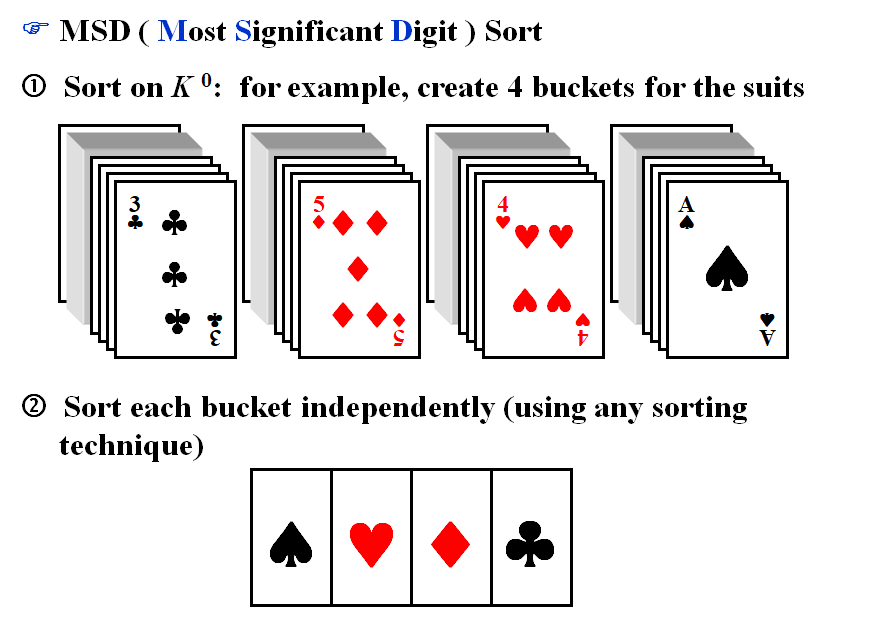
MSD(Most Significant Digit) Sort and LSD(Least Significant Digit) Sort

稳定的排序算法：冒泡排序、插入排序、归并排序、基数排序
不稳定的排序算法：选择排序、快速排序、希尔排序、堆排序

牢牢记住，归并、基数这两个看起来就比较稳，快排和希尔看起来就不稳

9-4

这里需要注意：希尔排序的平均情况是跟增量的选择有关系的，不能简单地认为是 $n\log n$ ，如果增量取得不好会退化成最差情况， $N^{\frac{3}{4}}$ 只是某个序列时候的最好情况；其最好情况是能达到 $O(n)$ 的，这是快排、堆排和归并做不到的；堆排、归并的三个量是一样的，都是 $n\log n$ ；快排和希尔的最坏能达到 $O(n^2)$ 。
空间上这张表里面写得有点问题，堆排和希尔不用额外的空间，是四个里面最好的；归并要开额外开一个 $N$ 的空间来暂时放已经排好的子列（先要分治再合并，合并的时候只能将两个并成一个），是四个里面最差的；快排自己就能排，但是需要递归实现，递归实现就要靠系统调用栈，深度是 $O(\log n)$ ，处于中间。

相当于是希尔 = 堆排 < 快排 < 归并
归并是学到现在的唯一一种可以作为外部排序的排序算法。

8 Hashing

8.1 General Idea

Symbol Table ADT

Objects : A set of name-attribute pairs, where the names are unique
Operations :
- SymTab Create(TableSize)
- Boolean IsIn(symtab, name)
- Attribute Find(symtab, name)
- SymTab Insert(symtab, name, attr)
- SymTab Delete(symtab, name)

Hash Tables

A collision occurs when we hash two nonidentical identifiers into the same bucket.
An overflow occurs when we hash a new identifier into a full bucket.

8.2 Hash Function

$f(x)$ must be easy to compute and minimize the number of collisions.
$f(x)$ should be unbiased. For any $x$ and any $i$ , we have that $Probability(f(x)=i)=\frac{1}{b}$ . Such kind of a hash function is called a uniform hash function.

8.3 Separate Chaining（链地址法）

keep a list of all keys that hash to the same value
链地址法的装填因子loading density和开放地址法是一样的，就是key的数量除以表长；但是其平均查找时间的算法和开放地址法的不一样。

9-2

而开放地址法就是把每个元素的查找次数加起来：

9-3

struct ListNode; 
typedef struct ListNode *Position; 
struct HashTbl; 
typedef struct HashTbl *HashTable; 
struct ListNode { 
    ElementType Element; 
    Position Next; 
}; 
typedef Position List; 
/* List *TheList will be an array of lists, allocated later */ 
/* The lists use headers (for simplicity), */ 
/* though this wastes space */ 
struct HashTbl { 
    int TableSize; 
    List *TheLists; 
};

Create an empty table

HashTable InitializeTable( int TableSize ) 
{   
    HashTable H; 
    int i; 
    if ( TableSize < MinTableSize ) 
    { 
        Error( "Table size too small" );  
        return NULL;  
    } 
    H = malloc( sizeof( struct HashTbl ) );  /*Allocate table*/
    if ( H == NULL ) FatalError( "Out of space!!!" ); 
    H->TableSize = NextPrime( TableSize );  /*Better be prime*/
    H->TheLists = malloc( sizeof( List )* H->TableSize );  /*Array of lists*/
    if ( H->TheLists == NULL ) FatalError( "Out of space!!!" );
    H->TheList = malloc(H->TableSize*sizeof(struct ListNode));
    for( i = 0; i < H->TableSize; i++ ) 
    {   /*Allocate list headers*/
        //H->TheLists[ i ] = malloc( sizeof( struct ListNode ) ); /* Slow! */
        if ( H->TheLists[ i ] == NULL ) FatalError( "Out of space!!!" ); 
        else H->TheLists[ i ]->Next = NULL;
    } 
    return H; 
}

Find a key from a hash table

Position Find ( ElementType Key, HashTable H ) 
{ 
    Position P; 
    List L; 
    L = H->TheLists[ Hash( Key, H->TableSize ) ]; 
    P = L->Next; 
    while( P != NULL && P->Element != Key )  /*Probably need strcmp*/ 
        P = P->Next; 
    return P; 
}

Insert a key into a hash table

void Insert ( ElementType Key, HashTable H ) 
{ 
    Position Pos, NewCell; 
    List L; 
    Pos = Find( Key, H ); 
    if ( Pos == NULL ) 
    {   /*Key is not found, then insert*/
        NewCell = malloc( sizeof( struct ListNode ) ); 
        if ( NewCell == NULL ) FatalError( "Out of space!!!" ); 
        else 
        { 
             L = H->TheLists[ Hash( Key, H->TableSize ) ]; /*Compute again is bad*/
             NewCell->Next = L->Next; 
             NewCell->Element = Key; /*Probably need strcpy!*/ 
             L->Next = NewCell; 
        } 
    } 
}

Note : Make the TableSize about as large as the number of keys expected (i.e. to make the loading density factor $\lambda\approx$1).

8.4 Open Addressing（开放地址法）

find another empty cell to solve collision(avoiding pointers)

Algorithm: insert key into an array of hash table
{
    index = hash(key);
    initialize i = 0 ------ the counter of probing;
    while (collision at index) 
    {
        index = (hash(key)+f(i))%TableSize; /*f(i) is collision resolving function*/
        if (table is full) break;
        else i++;
    }
    if (table is full) ERROR (“No space left”);
    else insert key at index;
}

Note : Generally $\lambda<0.5$ . 一般装填因子在0.5以下。

Linear Probing

$F(i)$ is a linear function of $i$ , such as $F(i)=i$ . 千万注意， $F(i)$ 是在原来的 $hash(key)$ 的基础上加的，别直接在 $key$ 的基础上加。
逐个探测每个单元(必要时可以绕回)以查找出一个空单元
使用线性探测的预期探测次数对于插入和不成功的查找来说大约是 $\frac{1}{2}(1+\frac{1}{(1-\lambda)^2})$ ，对于成功的查找来说是 $\frac{1}{2}(1+\frac{1}{1-\lambda})$ ，随着 $\lambda$ 变大会越来越差。
Cause primary clustering : any key that hashes into the cluster will add to the cluster after several attempts to resolve the collision.

注意：有的时候它给的除数和TableSize是完全不一样的两个数，别mod的时候想当然认为是一样的。

Quadratic Probing

$F(i)$ is a quadratic function of $i$ , such as $F(i)=i^2$ .

[Theorem] If quadratic probing is used, and the table size is prime, then a new element can always be inserted if the table is at least half empty. 考判断题！！

这个证明的意思就是说，最后如果 $i$ 和 $j$ 的和或者差要能整除TableSize，但是 $i\neq j$ ，而且它们的取值范围摆在那边，这就可以推得两次探测的肯定是不一样的。

Note : If the table size is a prime of the form $4k + 3$ , then the quadratic probing $f(i) = \pm i^2$ can probe the entire table. 能探测到表的每一个位置。

真正实操的时候一般是每次直接上 $ 2 \cdot i - 1$的

HashTable InitializeTable(int TableSize)
{
    HashTable H;
    int i;
    if(TableSize < MinTableSize)
    {
        Error("Table size too small");
        return NULL;
    }
    /*Allocate table*/
    H = malloc(sizeof(struct HashTbl));
    if(H == NULL)
        Fatal Error("Out of space!!!");
    H->TableSize = NextPrime(TableSize);
    
    /*Allocate array of Cells*/
    H->TheCells = malloc(sizeof(Cell)*H->TableSize);
    if(H->TheCells == NULL)
        FatalError("Out of space!!!");

    for(i = 0; i < H->TableSize; i++)
        H->TheCells[ i ].Info = Empty;
    return H;
}

Position Find(ElementType Key, HashTable H) 
{   
    Position CurrentPos; 
    int CollisionNum; 
    CollisionNum = 0; 
    CurrentPos = Hash(Key, H->TableSize); 
    while(H->TheCells[ CurrentPos ].Info != Empty &&
          H->TheCells[ CurrentPos ].Element != Key) 
    { 
        CurrentPos += 2*++CollisionNum-1; 
        if (CurrentPos >= H->TableSize)  
            CurrentPos -= H->TableSize;   /*Faster than mod*/
    } 
    return CurrentPos; 
}

void Insert(ElementType Key, HashTable H) 
{ 
    Position Pos; 
    Pos = Find(Key, H); 
    if (H->TheCells[ Pos ].Info != Legitimate) 
    { /*OK to insert here*/ 
        H->TheCells[ Pos ].Info = Legitimate; 
        H->TheCells[ Pos ].Element = Key; /*Probably need strcpy*/ 
    } 
}

Note :

Insertion will be seriously slowed down if there are too many deletions intermixed with insertions.

Although primary clustering is solved, secondary clustering occurs, that is, keys that hash to the same position will probe the same alternative cells.

Double Hashing（双重哈希）

$f(i)=i*hash_2(x)$
$hash_2(x)\not\equiv 0$
make sure that all cells can be probed
$hash_2(x)=R-(x\%R)$ with $R$ a prime smaller than TableSize, will work well.
比如说 $hash_1(x) \mod TableSize$ 冲突了，那么就上 $(hash_1(x) + hash_2(x)) \mod TableSize$ ，如果说键值不同的话，一般来说一次应该可以解决了；如果反复插入同一个键值，可能就要把 $hash_s(x)$ 翻倍了 $(hash_1(x) + 2hash_2(x)) \mod TableSize$ 了。

Note :

If double hashing is correctly implemented, simulations imply that the expected number of probes is almost the same as for a random collision resolution strategy.

Quadratic probing does not require the use of a second hash function and is thus likely to be simpler and faster in practice.

8.5 Rehashing（二次哈希）

Build another table that is about twice as big. (尽量选择一个比两倍大的而且是质数的数)
Scan down the entire original hash table for non-deleted elements.
Use a new function to hash those elements into the new table.
When to rehash
- As soon as the table is half full
- When an insertion fails
- When the table reaches a certain load factor

Note : Usually there should have been N/2 insertions before rehash, so O(N) rehash only adds a constant cost to each insertion. However, in an interactive system, the unfortunate user whose insertion caused a rehash could see a slowdown.

HashTable Rehash(HashTable H)
{
    int i, OldSize;
    Cell *OldCells;
    OldCells = H->TheCells;
    OldSize = H->TableSize;
    
    /*Get a new, empty table*/
    H = InitializeTable(2*OldSize);
    /*Scan through old table, reinserting into new*/
    for(i = 0; i < OldSize; i++)
        if(OldCells[i].Info == Legitimate)
            Insert(OldCells[i].Element, H);
    free(OldCells);
    
    return H;
}

1 Algorithm Analysis

[Definition] An algorithm is a finite set of instructions that, if followed, accomplishes a particular task. In addition, all algorithms must satisfy the following criteria.

[Example] Selection Sort : Sort a set of n≥1n\geq1n≥1 integers in increasing order

1.1 What to Analyze

[Example] Matrix addition

[Example] Iterative function for summing a list of numbers

[Example] Recursive function for summing a list of numbers

1.2 Asymptotic Notation(O,Ω,Θ,oO,\Omega,\Theta,oO,Ω,Θ,o)

[Definition] T(N)=O(f(N))T(N)=O(f(N))T(N)=O(f(N)) if there are positive constants ccc and n0n_0n0​ such that T(N)≤c⋅f(N)T(N)\leq c\cdot f(N)T(N)≤c⋅f(N) for all N≥n0N\geq n_0N≥n0​.(upper bound)

[Definition] T(N)=Ω(g(N))T(N)=\Omega(g(N))T(N)=Ω(g(N)) if there are positive constants ccc and n0n_0n0​ such that T(N)≥c⋅f(N)T(N)\geq c\cdot f(N)T(N)≥c⋅f(N) for all N≥n0N\geq n_0N≥n0​.(lower bound)

[Definition] T(N)=Θ(h(N))T(N)=\Theta(h(N))T(N)=Θ(h(N)) if and only if T(N)=O(h(N))T(N)=O(h(N))T(N)=O(h(N)) and T(N)=Ω(h(N))T(N)=\Omega(h(N))T(N)=Ω(h(N))

[Definition] T(N)=o(p(N))T(N)=o(p(N))T(N)=o(p(N)) if T(n)=O(p(N))T(n)=O(p(N))T(n)=O(p(N)) and T(N)≠Θ(p(N))T(N)\neq\Theta(p(N))T(N)​=Θ(p(N))

[Example] Matrix addition

General Rules

1.3 Compare the Algorithms

[Example] 最大子序列和

1.4 Logrithms in the Running Time

[Example] Binary Search

[Example] Euclid’s Algorithm

[Example] Efficient exponentiation

1.5 Checking Your Analysis

Method 1

Method 2

2 LIst, Stacks and Queues

2.1 Abstract Data Type(ADT) 抽象数据类型

[Definition] Data Type = {Objects} and {Operations}

[Definition] An Abstract Data Type(ADT) is a data type that is organized in such a way that the specification on the objects and specification of the operations on the objects are separated from the representation of the objects and the implementation on the operations.

2.2 The List ADT

Simple Array implementation of Lists

Linked Lists

Doubly Linked Circular Lists

Two Applications

Cursor Implementation of Linked Lists(no pointer)

2.3 The Stack ADT

Linked List Implementation (with a header node)

Array Implementation of Stacks

Application

2.4 The Queue ADT

Array Implementation of Queues

3 Trees

3.1 Preliminaries

[Definition] A tree is a collection of nodes. The collection can be empty; otherwise, a tree consists of (1) a distinguished node r, called the root; (2) and zero or more nonempty (sub)trees, each of whose roots are connected by a directed edge from r.

Terminologies

List Representation

FirstChild-NextSibling Representation

3.2 Binary Trees

[Definition] A binary tree is a tree in which no node can have more than two children.

Tree Traversals (visit each node exactly once)

Threaded Binary Trees

Properties of Binary Trees

3.3 Binary Search Trees

[Definition] A binary search tree is a binary tree. It may be empty. If it is not empty, it satisfies the following properties:

ADT

Implementations

4 Priority Queues (Heaps)

4.1 ADT Model

4.2 Implementations

Array

Linked List

Ordered Array

Ordered Linked List

Binary Search Tree

4.3 Binary Heap

Structure Property

Heap Order Property

Basic Heap Operations

Other Heap Operations

4.4 Applications of Priority Queues

Heap Sort

查找一个序列中第k小的元素

4.5 ddd-Heaps — All nodes have ddd children

5 The Disjoint Set

5.1 Equivalence Relations

[Definition] A relation R is defined on a set S if for every pair of elements (a, b), a, b ∈\in∈ S, a R b is either true or false. If a R b is true, then we say that a is related to b.

[Definition] A relation, ~, over a set, S, is said to be an equivalence relation over S if it is symmetric, reflexive, and transitive over S.

[Definition] Two members x and y of a set S are said to be in the same equivalence class if x ~ y.

5.2 The Dynamic Equivalence Problem

5.3 Basic Data Structure

Union( i,ji, ji,j )

Find( iii )

[Example] Selection Sort : Sort a set of $n\geq1$ integers in increasing order

1.2 Asymptotic Notation( $O,\Omega,\Theta,o$ )

[Definition] $T(N)=O(f(N))$ if there are positive constants $c$ and $n_0$ such that $T(N)\leq c\cdot f(N)$ for all $N\geq n_0$ .(upper bound)

[Definition] $T(N)=\Omega(g(N))$ if there are positive constants $c$ and $n_0$ such that $T(N)\geq c\cdot f(N)$ for all $N\geq n_0$ .(lower bound)

[Definition] $T(N)=\Theta(h(N))$ if and only if $T(N)=O(h(N))$ and $T(N)=\Omega(h(N))$

[Definition] $T(N)=o(p(N))$ if $T(n)=O(p(N))$ and $T(N)\neq\Theta(p(N))$

4.5 $d$ -Heaps — All nodes have $d$ children

[Definition] A relation R is defined on a set S if for every pair of elements (a, b), a, b $\in$ S, a R b is either true or false. If a R b is true, then we say that a is related to b.

Union( $i, j$ )

Find( $i$ )

[Definition] A topological order is a linear ordering of the vertices of a graph such that, for any two vertices, $i$ , $j$ , if $i$ is a predecessor of $j$ in the network then $i$ precedes $j$ in the linear ordering.

[Definition] A spanning tree of a graph $G$ is a tree which consists of $V(G)$ and a subset of $E(G)$